arcov
The parameters of the autoregression model with all poles are the covariance method.
| Library |
|
Syntax
Function call
-
a,e = arcov(x,p)— returns normalized autoregression parameters (AR)a, corresponding order modelspfor the input arrayx, wherexIt is assumed to be the output of an AR system controlled by white noise. This method minimizes the error of direct prediction using the least squares method.It also returns the calculated variance.
einput white noise.
Arguments
Examples
Estimation of parameters using the covariance method
Details
We use the vector of coefficients of the polynomial to generate the autoregression process. 4-th order by filtering 1024 white noise samples. Reset the random number generator to get reproducible results. We use the covariance method to estimate the coefficients.
import EngeeDSP.Functions: randn,filter,arcov

A = [1 -2.7607 3.8106 -2.6535 0.9238]
y = filter(1,A,0.2*randn(1024,1))
arcoeffs = arcov(y,4)[1]
1×5 Matrix{Float64}:
1.0 -2.77456 3.8419 -2.68565 0.936713Generate 50 implementations of the process, changing the variance of the input noise each time. Let’s compare the variance calculated using covariance with the actual values.
nrealiz = 50
order = 4
noisestdz = rand(1, nrealiz) .+ 0.5
randnoise = randn(1024, nrealiz)
noisevar = zeros(1, nrealiz)

for k in 1:nrealiz
    y = filter(ones(1), A, noisestdz[k] * randnoise[:, k])
        arcoeffs,noisevar[k] = arcov(y, order)

end

p=scatter(vec(noisestdz.^2), vec(noisevar),
        marker=:x,
        markerstrokecolor=:blue,
        xlabel="Input",
        ylabel="Estimated",
        title="Noise Variance",
        label="Single channel loop",
        legend=false)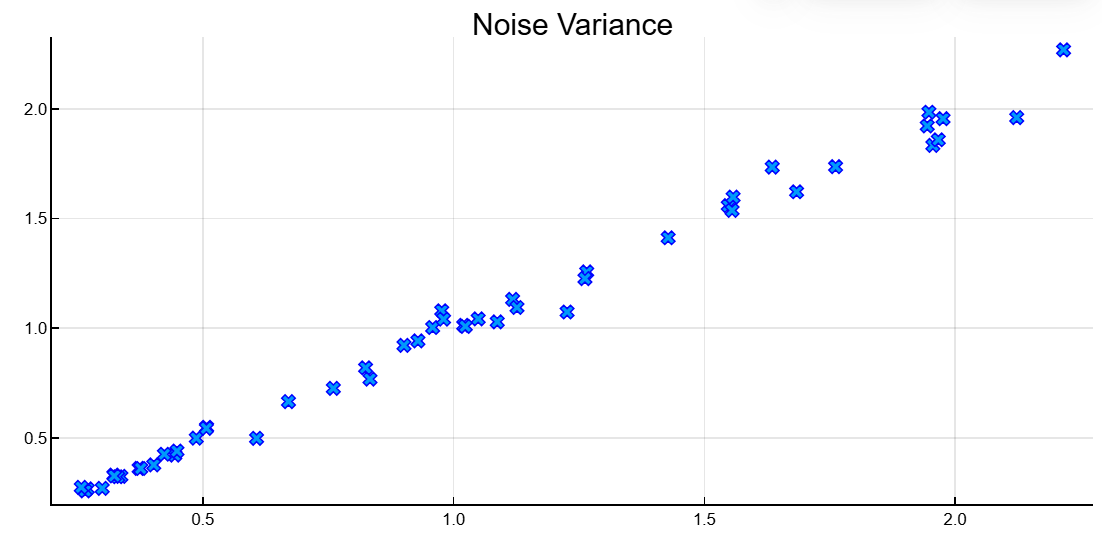
Let’s repeat the procedure using the multi-channel syntax of the function.
Y = filter(1,A,noisestdz.*randnoise)

coeffs,variances = arcov(Y,4)

scatter!(p,noisestdz.^2, variances,
        marker=:circle,
        markercolor=:transparent,
        markerstrokecolor=:green,
        markersize=10)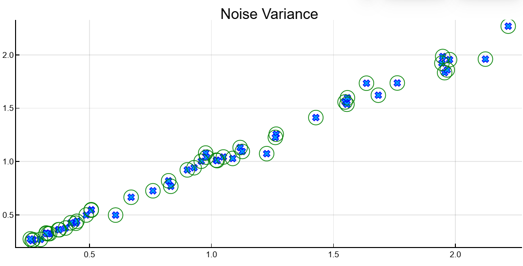
Additional Info
An autoregression model of the order of p
Details
In the autoregression model of the order ( ) the current output is a linear combination of the previous ones outputs plus a white noise input signal. Weights on previous ones The outputs minimize the average quadratic error of the autoregression prediction.
Let a stationary, broadly random process obtained by filtering the white noise of the variance using the system function . If — spectral power density , then
Since the covariance method characterizes the input data using a model with all poles, the correct choice of the model order is very important.