lpc
Coefficients of the linear predictive filter.
| Library |
|
Syntax
Function call
-
a,g = lpc(x,p)— finds coefficients of the linear predictor of the orderp, FIR filter that predicts the current value of a real time seriesxbased on past counts. The function also returns the variance of the prediction error.g. Ifxis a matrix, then the function treats each column as an independent channel.
Arguments
Input arguments
# x — input array
+
vector | the matrix
Details
An input array specified as a vector or matrix. If x is a matrix, then the function treats each column as an independent channel.
Output arguments
# g is the variance of the prediction error
+
scalar | vector
Details
The variance of the prediction error returned as a scalar or vector.
Examples
Estimation of time series using the direct prediction method
Details
Let’s evaluate a series of data using a third-order direct predictor. Let’s compare the estimate with the original signal.
First, we will create the signal data as the output of an autoregressive (AR) process controlled by normalized white Gaussian noise. We use the latest ones 4096 counts the output data of the AR process to avoid transients during startup.
import EngeeDSP.Functions: randn, filter, lpc, xcorr

noise = randn(50000,1)
x = filter(1,[1 1/2 1/3 1/4],noise)
x = x[end-4096+1:end]
Calculate the predictor coefficients and the estimated signal.
a,g = lpc(x, 3)
est_x = filter([0; -a[2:end]], 1, x)
Let’s compare the predicted signal with the original signal by plotting the latter 100 counts of each signal.
plot(1:100, x[end-99:end], label="Original signal", linewidth=1)
plot!(1:100, est_x[end-99:end], label="LPC estimate", linestyle=:dash, linewidth=1)

plot!(xlabel="Sample Number", ylabel="Amplitude")
plot!(grid=true)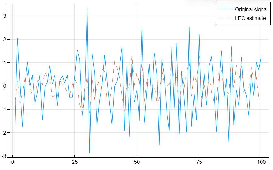
Calculate the prediction errors and the autocorrelation sequence of prediction errors. Let’s plot the autocorrelation graph. The prediction error is approximately white Gaussian noise, as expected for the input process of the third-order autoregressive model.
e = x-est_x
acs,lags = xcorr(e,"coeff")

plot(lags', acs)
plot!(xlabel="Lags", ylabel="Normalized Autocorrelation")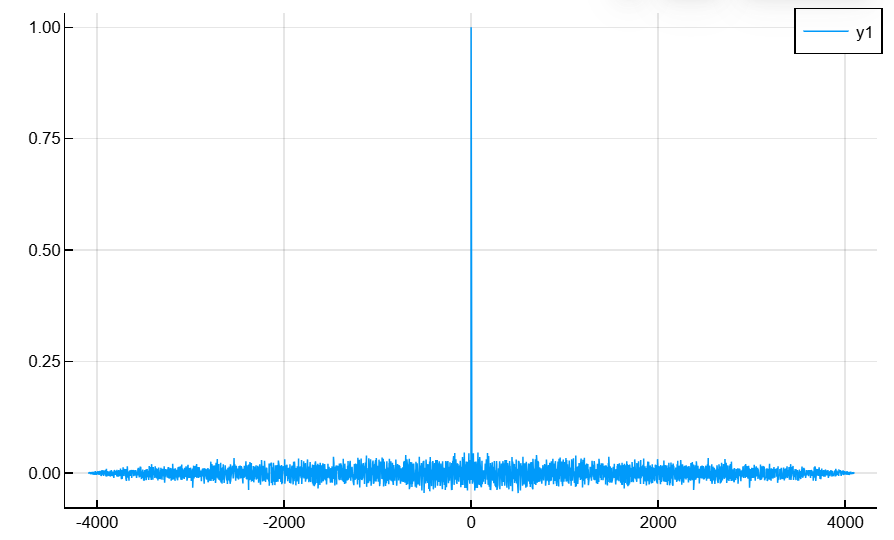

Algorithms
Function lpc determines the coefficients of a direct linear predictor, minimizing the prediction error using the least squares method. It finds application in filter design and speech encoding.
Function lpc Uses the autocorrelation autoregression (AR) modeling method to find the filter coefficients. The generated filter may not accurately simulate the process, even if the sequence of data is indeed an AR process of the correct order, since the autocorrelation method implicitly encloses the data in a window. In other words, the method assumes that the samples of the signal are beyond the length x equal 0.
Function lpc calculates the least squares solution for , where
and — length . Solving the least squares problem using normal equations leads to the Yule—Walker equations: