Comparison of Julia and MATLAB performance on matrix operations

We present the results of a computational experiment: estimates of how many times performing matrix operations on Julia allows you to speed up the code relative to the same operations in MATLAB.

Let's start by preparing the environment. We will install libraries that may not be included in the standard Engee package at the time of publication, then connect the necessary libraries and switch the graphics output core to non-interactive mode.

]add BenchmarkTools StatsPlots

using BenchmarkTools, LinearAlgebra, MATLAB, StatsPlots
gr()

For information, let's compare the versions of the libraries used by both systems to perform matrix operations. There are many library implementations for matrix operations. As a rule, the set of these functions is collectively called BLAS (Basic Linear Algebra Subroutines, basic linear algebra routines) and the use of one or another implementation optimized for certain processors may be one of the comparison factors.

mat"version -blas"

"Intel(R) oneAPI Math Kernel Library Version 2024.1-Product Build 20240215 for Intel(R) 64 architecture applications (CNR branch auto)"

mat"maxNumCompThreads()"

48.0

Not only do MATLAB and Julia have different implementations of BLAS, but also the number of threads.:

BLAS.get_config()

LinearAlgebra.BLAS.LBTConfig
Libraries: 
└ [ILP64] libopenblas64_.so

BLAS.vendor()

:lbt

BLAS.get_num_threads()

24

BLAS.set_num_threads(48)

BLAS.get_num_threads()

48

We see that MATLAB uses Intel's oneAPI library, and Julia uses the libopenblas64 opensource library. On the Engee side, both systems have been allocated the same resources for testing. We can start the comparison.

The matrix multiplication problem

Let's solve the Julia problem by saving all the execution results into a vector (we will output only the median results):

sizes = Int.([0.5e2, 1e2, 0.5e3, 1e3, 0.5e4, 1e4])

julia_times = []
for n in sizes
    result = @benchmark rand($n,$n) * rand($n,$n);
    append!(julia_times, [result.times ./ 1e9]) # ns to sec
end

# Let's output the median time for each launch for verification
median.(julia_times)

6-element Vector{Float64}:
  2.2984e-5
  0.000101845
  0.428853208
  0.699654599
 12.763432786
 58.412450882

We could save the median time by the command Float64(median(result.times) / 1e9)) but it would be interesting to see graphs with tolerances, so we save all the results. Now let's solve the problem on the MATLAB core, which is available to us.:

@mput sizes                                   # Transfer matrix parameters to MATLAB

mat"""
run_times = [];
for i = 1:length(sizes)
    n = sizes(i);
    TestFunc = @() rand(n, n) * rand(n, n); % Define the function for testing
    t = timeit(TestFunc); % We measure the execution time
    run_times = [run_times, t]; % is saved to the output vector
end
""";

matlab_time = @mget run_times                # Get a vector of results from MATLAB

1×6 Matrix{Float64}:
 0.000382712  0.000934712  0.0156977  0.100696  5.25263  31.8614

How is the environment @benchmark in Julia, so is the function timeit in MATLAB, both run the operation being transferred to multiple times.

Let's build a graph that will show how much acceleration Julia allows us to achieve.:

n_points = length(sizes)
julia_means = zeros(n_points)
julia_stds = zeros(n_points)
for i in 1:n_points
    julia_means[i] = mean(julia_times[i])
    julia_stds[i] = std(julia_times[i])
end
data_matrix = [julia_means matlab_time']

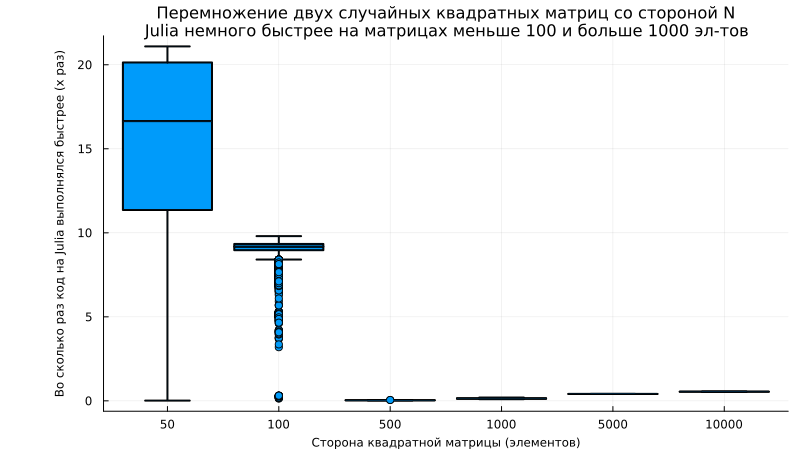
boxplot([matlab_time[i]./julia_times[i] for i in 1:length(sizes)], c=1, legend=false,
      xlabel="The side of the square matrix (elements)", ylabel="How many times did the Julia code run faster (x times)",
      xticks=(1:length(sizes),sizes), lw=2, guidefont=font(8), left_margin=15Plots.mm, size=(800,450),
      title="Multiplication of two random square matrices with the N\nJulia side is slightly faster on matrices less than 100 and more than 1000 elements", titlefont=font(11))

The problem of exponentiation

Let's measure the execution time in Julia and in MATLAB:

sizes = Int.([0.5e2, 1e2, 0.5e3, 1e3, 0.5e4, 1e4])

# Measurement in Julia
julia_times = []
for n in sizes
    A = rand(n,n);
    result = @benchmark $A .^3;
    append!(julia_times, [result.times ./ 1e9]) # ns to sec
end

@mput sizes                         # Transfer matrix parameters to MATLAB
mat"""
run_times = [];
for i = 1:length(sizes)
    n = sizes(i);
    A = rand(n, n); % Creating a random matrix
    testFunc = @() A .^ 3; % Defining the function for testing
    t = timeit(TestFunc); % We measure the execution time
    run_times = [run_times, t]; % is saved to the output vector
end
""";
matlab_time = @mget run_times;      # Get a vector of results from MATLAB

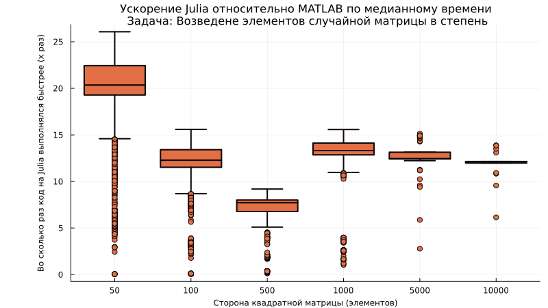
Let's build a graph that will show how much faster matrix multiplication can be achieved using Julia.:

boxplot([matlab_time[i]./julia_times[i] for i in 1:length(sizes)], c=2, legend=false,
      xlabel="The side of the square matrix (elements)", ylabel="How many times did the Julia code run faster (x times)",
      xticks=(1:length(sizes),sizes), lw=2, guidefont=font(8), titlefont=font(11),
      title="Julia acceleration relative to MATLAB in median time\n Task: Raising the elements of a random matrix to a power", left_margin=15Plots.mm, size=(800,450))

The problem of matrix multiplication

Similarly to the previous examples, we perform matrix multiplication:

sizes = Int.([.5e2, 1e2, .5e3, 1e4, .5e5])

# Measurement in Julia
julia_times = []
for n in sizes
    A = rand(n,n); B = rand(n,n);
    result = @benchmark $A * $B;
    append!(julia_times, [result.times ./ 1e9]) # ns to sec
end

@mput sizes                          # Transfer matrix parameters to MATLAB
mat"""
run_times = [];
for i = 1:length(sizes)
    n = sizes(i);
    A = rand(n, n); B = rand(n, n); % Creating random matrices
    testFunc = @() A * B; % Defining the function for testing
    t = timeit(TestFunc); % We measure the execution time
    run_times = [run_times, t]; % is saved to the output vector
end
""";
matlab_time = @mget run_times;       # Get a vector of results from MATLAB

boxplot([matlab_time[i]./julia_times[i] for i in 1:length(sizes)], c=3, legend=false,
      xlabel="The side of the square matrix (elements)", ylabel="How many times did the Julia code run faster (x times)",
      xticks=(1:length(sizes),sizes), lw=2, guidefont=font(8), titlefont=font(11),
      title="Julia acceleration relative to MATLAB in median time\n Task: Raising the elements of a random matrix to a power", left_margin=15Plots.mm, size=(800,450))

Conclusion

In addition to the visual conclusions presented in the graphs, we can see how easy it is to compare the execution of functions in MATLAB and Julia and draw our own conclusions.

Share your opinion – did we spoil the test results with some suboptimal approach, and suggest your options for functions!