gmonopuls
Gaussian monopulse.
| Library |
|
Arguments
Input arguments
# t — time values
+
vector
Details
The time values at which a Gaussian monopulse with a single amplitude is calculated, specified as a vector.
# fc — carrier frequency
+
1000 (by default) | scalar
Details
The carrier frequency in Hz, set as a real positive scalar. By default fc = 1000 Hz.
Examples
Gaussian monopulse
Details
Consider a Gaussian mono pulse with a carrier frequency GHz and sampling rate GHz. Let’s determine the cutoff time using the option "cutoff" and calculate the monopulse in the range of before .
import EngeeDSP.Functions: gmonopuls

fc = 2e9
fs = 100e9

tc = gmonopuls("cutoff", fc)
t = -2*tc:1/fs:2*tc

y = gmonopuls(t, fc)
The monopulse is determined by the equation:
where , and the exponential multiplier is such that . Let’s plot two curves and make sure that they coincide.
using Plots

sg = 1/(2*pi*fc)
ys = exp(1/2) * t/sg .* exp.(-(t/sg).^2/2)

plot(t, y, label="gmonopuls")
scatter!(t, ys, markershape=:circle, label="Definition")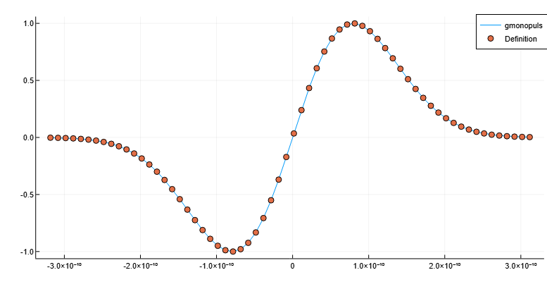
A sequence of Gaussian monopulses
Details
Consider a Gaussian mono pulse with a carrier frequency GHz and sampling rate GHz. We use this monopulse to build a sequence of pulses with an interval between them. 7.5 hc. Let’s determine the cutoff time for each pulse using the option "cutoff". Let’s set the delay times multiples of the interval between pulses.
import EngeeDSP.Functions: gmonopuls
import EngeeDSP.Functions: pulstran

fc = 2e9
fs = 100e9

tc = gmonopuls("cutoff", fc)
D = [2.5, 10.0, 17.5] * 1e-9
We will generate a sequence of pulses with a total duration C. Let’s display the result on the graph.
using Plots

t = 0:1/fs:150*tc
yp = pulstran(t, D, "gmonopuls", fc)

plot(t, yp)