pwelch
Estimation of the spectral density of Welch power.
| Library |
|
Syntax
Function call
-
pxx,f,pxxc = pwelch(x,out=:data)— returns an estimate of the spectral power density (SPM) of the signalx, calculated by averaging the overlapping Welch segments. ColumnsxThey are considered as independent channels. It also returns frequenciesfin rad/count and confidence interval boundspxxcwith a level95% by default.
-
pxx,f,pxxc = pwelch(___,freqRange,spectrumType,trace,out=:data)— additionally sets the frequency rangefreqRange, spectrum typespectrumTypeand the tracing modetrace. You can specify any of the previous input syntax options.
-
pxx,f,pxxc = pwelch(___,Name,Value,out=:data)— sets additional parameters using arguments like «name-value» for any of the previous syntax options.
-
pwelch(___)— plots the estimation of the SPM or the Welch power spectrum.
Arguments
Input arguments
# x — input signal
+
vector | the matrix
Details
An input signal specified as a vector or matrix. If x — matrix, function pwelch considers its columns as independent channels.
| Типы данных |
|
| Support for complex numbers |
Yes |
# win — window
+
empty array (default) | an integer | vector
Details
A window set as an empty array Float32[], Float64[] or Int64[], a positive integer or vector.
Function pwelch divides the input signal x divides into segments and applies a window to incrementally multiply the counts of each segment by the window values. The window values depend on the way this argument is set.:
-
Float32[],Float64[]orInt64[]— the function applies a Hamming window of such length to splitxon8segments with overlap innOverlapcounts; -
a positive integer— the function dividesxinto segments of lengthwinand applies a Hamming window of the same length; -
vector— the function dividesxinto segments of length equal to the length of the vectorwin, and applies the window specified in the argumentwin.
If the length is x does not allow you to get an integer number of overlapping segments nOverlap counts, function pwelch truncates the signal accordingly x.
For a list of available windows, see in the library Spectral analysis.
By default, the Hamming window has a weakening of the side lobes at the level of 42.5 dB, so the spectral components are below this level (relative to the maximum component) they can be hidden. Selecting a different window allows you to change the ratio between resolution (for example, using a rectangular window) and attenuation of the side lobes (for example, using a Hanna window).
|
| Типы данных |
|
# nOverlap — number of overlapping counts
+
empty array (by default) | an integer
Details
The number of overlapping samples set as an empty array Float32[], Float64[] or Int64[] or a non-negative integer.
-
Float32[],Float64[]orInt64[]— the function selects a value that ensures that the segments overlap on50%.If the segment length is not specified, the function sets the value for this argument. , where — the length of the input signal, and denotes the rounding down function. This action is equivalent to dividing the signal into as long segments as possible in order to get as many as possible, but no more than eight overlapping segments.
50%. -
A non-negative integer— adjacent segments overlap by the number of samples specified in this argument.
# freqSpec — frequency response
+
empty array (by default) | an integer | vector
Details
The frequency response specified in one of the following ways:
-
Float32[],Float64[]orInt64[]— the function calculates spectral estimates using the number of DFT points equal to the largest of the values256and the nearest power of two, equal to or greater than the window length; -
a positive integer— the function calculates spectral estimates using the number of DFT points specified in this argument:-
if
freqSpeclonger segment length, functionpwelchadds zeros to segment data; -
if
freqSpecless than the segment length, the function splits the segment modulofreqSpecand summarizes the resulting fragments;
-
-
vector, containing at least two elements, — the function calculates spectral estimates at the frequencies specified in this argument:
| Типы данных |
|
#
Fs — sampling
rate
scalar
Details
The sampling rate, set as a positive scalar. It is equal to the number of counts per unit of time. If time is measured in seconds, the sampling rate is expressed in Hz.
-
If the argument is
Fsset asFloat32[],Float64[]orInt64[], functionpwelchaccepts the sampling frequency of the input signalxequal1Hz. -
If the argument is
Fsnot specified, functionpwelchaccepts the sampling frequency equal to2πrad/countdown.
# freqRange — frequency range for estimating SPM or power spectrum
+
"onesided" | "twosided" | "centered"
Details
The frequency range of the SPM estimate or the power spectrum, defined as "onesided", "twosided" or "centered".
Function pwelch returns pxx with the number of rows and the frequency range depending on the value freqRange, the parity of the number of DFT points in freqSpec and it depends on whether the argument is set. Fs.
|
|
Number of lines in |
Frequency range for |
|
|
|
|||
|
Even number |
|
|
|
Odd number |
|
|
|
|
|
Even or odd |
|
|
|
|
Even number |
|
|
|
Odd number |
|
|
||
|
| Типы данных |
|
# spectrumType — scaling of the power spectrum
+
"psd" (by default) | "power"
Details
Scaling of the power spectrum, set to one of the following values:
-
"psd"— functionpwelchreturns the spectral power density; -
"power"— the function scales each SPM estimate by the equivalent noise frequency band of the window and returns an estimate of the power at each frequency.
The table shows the scaling ratio between the SPM estimate and the estimate of the power spectrum returned to pxx, with the specified input signal x, the window vector win, the length of the overlap nOverlap, frequency response freqSpec and the sampling rate Fs.
| Sampling rate | The scaling ratio |
|---|---|
|
Then |
|
Then |
# trace — trace mode
+
"mean" (default) | "maxhold" | "minhold"
Details
The trace mode set by one of the following values:
-
"mean"— functionpwelchreturns an estimate of the Welch spectrum for each input channel by averaging the estimates of the power spectrum of all segments in each frequency range; -
"maxhold"— the function returns the maximum retention spectrum for each input channel, selecting the maximum value of the power spectrum by segment in each frequency range; -
"minhold"— the function returns the minimum retention spectrum for each input channel, selecting the minimum value of the power spectrum by segment in each frequency range.
Input arguments «name-value»
Specify optional argument pairs as Name,Value, where Name — the name of the argument, and Value — the appropriate value. Type arguments «name-value» they should be placed after the other arguments, but the order of the pairs does not matter. You can specify multiple pairs «name-value».
Use commas to separate the name and value, and Name enclose it in quotation marks, or use an equal sign to separate the name and value, and Name specify it without quotation marks.
# ConfidenceLevel — confidence interval for the assessment of SPM
+
0.95 (by default) | scalar
Details
The coverage probability for the SPM estimate, given as a scalar in the range (0, 1).
If specified ConfidenceLevel = p (or "ConfidenceLevel", p),
function pwelch returns in the output argument pxxc the lower and upper bounds of the confidence interval with the level p × 100% for true SPM.
# Parent — the target parent container
+
empty array (default) | object Axes | object Panel
Details
The target parent container, set as an object Axes or Panel.
If specified Parent = h (or "Parent", h), function pwelch plots the estimation of the SPM or the Welch power spectrum on the specified target parent container, regardless of the presence of output arguments.
# out — type of output data
+
:plot (by default) | :data | :all
Details
Type of output data:
-
:plot— the function returns a graph; -
:data— the function returns data; -
:all— the function returns data and a graph.
| For this argument, the name and value are separated by an equal sign (=). |
Output arguments
# pxx — SPM score or power spectrum
+
vector | the matrix
Details
The SPM estimate or power spectrum returned as a real non-negative column vector or matrix.
-
Each column
pxxIt represents an estimate of the SPM or the power spectrum of the corresponding column.xdepending on how the argument is setspectrumType. -
The measurement units of the SPM estimate are the squares of the input signal value per unit frequency. For example, if the input data is
xset in volts, sampling rateFs— in hertz, and the resistance is1Ohms, then the SPM estimate will be expressed in Watts/Hz. -
The units of measurement of the power spectrum are the squares of the input signal. For example, if the input data is
xThey are set in volts, and the resistance is1Ohms, then the SPM estimate will be expressed in watts.
# f — frequencies associated with the assessment of SPM
+
vector
# pxxc — confidence intervals
+
the matrix
Details
The bounds of the confidence intervals returned as a real matrix.
-
The matrix
pxxchas as many rows aspxx. -
The matrix
pxxcit has twice as many columns aspxx.-
The odd columns contain the lower bounds of the confidence intervals.
-
The even columns contain the upper bounds of the confidence intervals.
Thus,
pxxc[m, 2 * n − 1]— this is the lower limit of the confidence interval, andpxxc[m, 2 * n]— the upper limit of the confidence interval corresponding to the estimatepxx[m, n]. -
-
The probability of covering confidence intervals is determined by the value of the argument
ConfidenceLevel.
| Типы данных |
|
Examples
Welch estimation using default input data
Details
We obtain an estimate of the Welch SPM for the input signal, which is a discrete sinusoid with an angular frequency rad/count and additive white noise .
Let’s create a sinusoid with an angular frequency rad/count and additive white noise . Reset the state of the random number generator to get reproducible results. The length of the signal is counts.
using Random
Random.seed!(0)

n = 0:319
x = cos.(π/4 * n) + randn(length(n))
We obtain an estimate of Welch’s SPM using the Hamming window and the default DFT length. The default segment length is 71 the count, and the length of the DFT contains 256 points, which gives frequency resolution rad/countdown. Since the signal is real, the SPM estimate is one-sided, and there is 256 / 2 + 1 points.
import EngeeDSP.Functions: pwelch

pxx, f, pxxc = pwelch(x, out = :data)
([0.1863630724000894; 0.33918260379618265; … ; 0.24304012258269603; 0.11708917663794487;;], [0.0; 0.02454369260617026; … ; 3.117048960983623; 3.141592653589793;;], [0.08146885100079476 0.7719778085293696; 0.1818050422612173 0.8436289786035511; … ; 0.130271774739574 0.6044994291550672; 0.05118568052389489 0.48502229985464423])Let’s build a graph of Welch’s SPM assessment.
pwelch(x)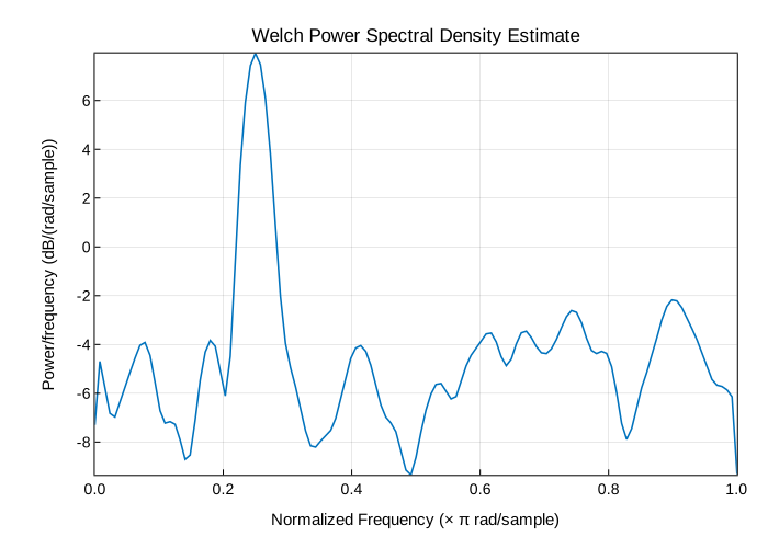
Let’s repeat the calculations.
-
Divide the signal into sections of length . This action is equivalent to dividing the signal into as long segments as possible in order to get as many as possible, but no more than 8 overlapping segments.
50%. -
We use the Hamming window for the segments.
-
Specify the overlap
50% between adjacent segments. -
To calculate the FFT, we use points where .
Let’s make sure that both approaches produce identical results.
Nx = length(x)
nsc = floor(Int, Nx / 4.5)
nov = floor(Int, nsc / 2)
nff = max(256, 2^nextpow(2, nsc))

import EngeeDSP.Functions: hamming

pxxt = pwelch(x, hamming(nsc), nov, nff, out = :data)

maxerr = maximum(abs.(abs.((pxxt[1])[:]) - abs.(pxx[:])))0.0Divide the signal into 8 equal overlapping segments 50% between them. We will specify the same length of the FFT as in the previous step. Let’s calculate Welch’s SPM score and make sure that the result matches the previous estimates.
ns = 8
ov = 0.5
lsc = Int(floor(Nx / (ns - (ns - 1) * ov)))

pxxt8 = pwelch(x, lsc, floor(ov * lsc), nff, out = :data)

maxerr8 = maximum(abs.(abs.((pxxt8[1])[:]) - abs.(pxx[:])))0.0Welch score with a given segment length
Details
We obtain an estimate of the Welch SPM for the input signal, which is a discrete sinusoid with an angular frequency rad/count and additive white noise .
Let’s create a sinusoid with an angular frequency rad/count and additive white noise . Reset the state of the random number generator to get reproducible results. The signal contains 512 counts.
using Random
Random.seed!(0)

n = 0:511
x = cos.(π/3 * n) + randn(length(n))
We obtain an estimate of Welch’s SPM by dividing the signal into segments of length 132 the countdown. The signal segments are multiplied by a Hamming window of length 132 the countdown. The number of overlapping counts is not specified, so it is set to 132 / 2 = 66. The length of the DFT is 256 points, which gives frequency resolution 2π / 256 rad/countdown. Since the signal is real, the SPM estimate is one-sided, and there is 256 / 2 + 1 = 129 points. Let’s plot the SPM as a function of the normalized frequency.
import EngeeDSP.Functions: pwelch

segmentLength = 132
pxx, w, pxxc = pwelch(x, segmentLength, out = :data)

plot(w/π, 10 * log10.(pxx),
     xlabel = "Normalized Frequency (× π rad/sample)",
     title = "Welch Power Spectral Density Estimate")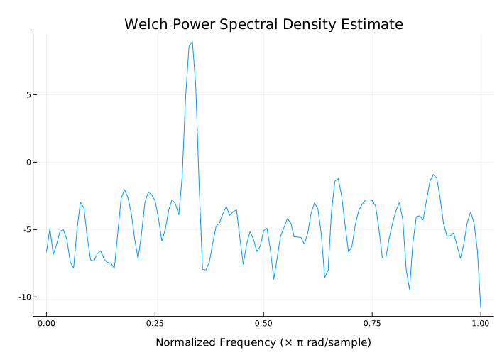
Welch score with a given segment overlap
Details
We obtain an estimate of the Welch SPM for the input signal, which is a discrete sinusoid with an angular frequency rad/count and additive white noise .
Let’s create a sinusoid with an angular frequency rad/count and additive white noise . Reset the state of the random number generator to get reproducible results. The length of the signal is 320 counts.
using Random
Random.seed!(0)

n = 0:319
x = cos.(π/4 * n) + randn(length(n))
We obtain an estimate of Welch’s SPM by dividing the signal into segments of length 100 counts. The signal segments are multiplied by a Hamming window of length 100 counts. The number of overlapping counts is 25. The length of the DFT is 256 points, which gives frequency resolution 2π / 256 rad/countdown. Since the signal is real, the SPM estimate is one-sided, and there is 256 / 2 + 1 points.
import EngeeDSP.Functions: pwelch

segmentLength = 100
noverlap = 25
pxx, f, pxxc = pwelch(x, segmentLength, noverlap, out = :data)

plot(10 * log10.(pxx),
     xlabel = "Frequency Samples",
     title = "Welch Power Spectral Density Estimate")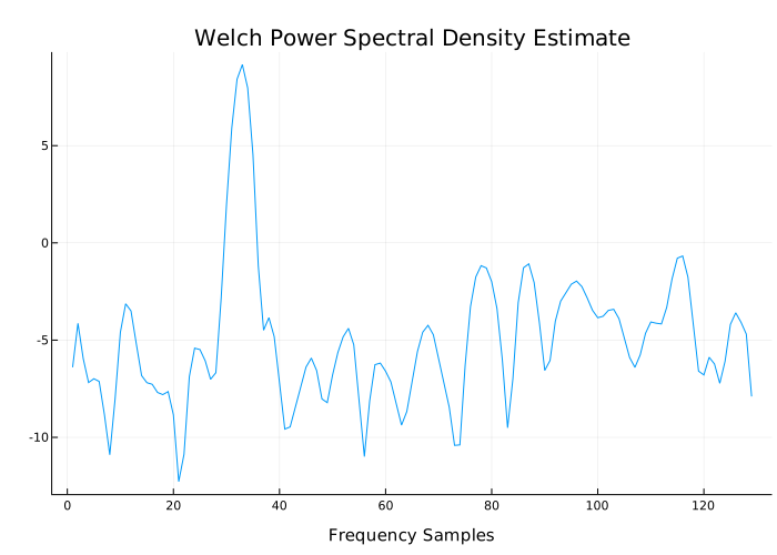
Welch estimation with a given DFT length
Details
We obtain an estimate of the Welch SPM for the input signal, which is a discrete sinusoid with an angular frequency rad/count and additive white noise .
Let’s create a sinusoid with an angular frequency rad/count and additive white noise . Reset the state of the random number generator to get reproducible results. The length of the signal is 320 counts.
using Random
Random.seed!(0)

n = 0:319
x = cos.(π/4 * n) + randn(length(n))
We obtain an estimate of Welch’s SPM by dividing the signal into segments of length 100 counts with overlap by default 50%. We specify the length of the DFT equal to 640 points, so that the frequency π/4 The rad/count corresponded to the 81st bin of the DFT. Since the signal is real, the SPM estimate is one-sided, and there is 640 / 2 + 1 points.
import EngeeDSP.Functions: pwelch

segmentLength = 100
nfft = 640
pxx, f, pxxc = pwelch(x, segmentLength, [], nfft, out = :data)

plot(10 * log10.(pxx),
     xlabel = "Frequency Points",
     title = "Welch Power Spectral Density Estimate")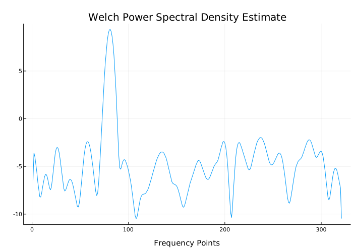
Estimation of the SPM signal using the Welch method with a frequency in Hz
Details
Let’s create a signal consisting of a sine wave with a frequency of 100 Hz in additive white noise . Reset the state of the random number generator to get reproducible results. The sampling rate is 1 kHz, the duration of the signal — 5 seconds.
using Random
Random.seed!(0)

Fs = 1000
t = 0:1/Fs:5-1/Fs
x = cos.(2π * 100 * t) + randn(length(t))
We obtain an estimate of the Welch SPM averaged over overlapping segments for the previous signal. Using the segment length 500 overlapping counts 300 counts. We use 500 DFT points so that the frequency 100 Hz fell directly into the DFT bin. Let’s enter the sampling frequency to get the frequency vector in Hz. Let’s plot the result graph.
import EngeeDSP.Functions: pwelch

pxx, f, pxxc = pwelch(x, 500, 300, 500, Fs, out = :data)

plot(f, 10 * log10.(pxx),
     xlabel = "Frequency (Hz)",
     ylabel = "PSD (dB/Hz)")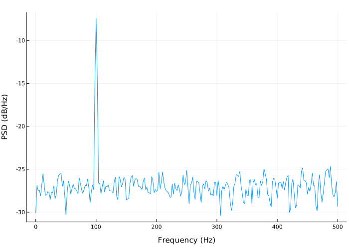
Upper and lower bounds of the confidence interval
Details
This example illustrates the use of confidence bounds with the SPM estimation method of averaging overlapping Welch segments. Although this is not a necessary condition for statistical significance, the frequencies in the Welch estimate, where the lower confidence limit exceeds the upper confidence limit for the surrounding estimates of the SPM, clearly indicate significant fluctuations in the time series.
Let’s create a signal consisting of a superposition of sinusoids with frequency 100 Hz and 150 Hz in additive white noise . The amplitude of the two sine waves is 1. The sampling rate is 1 kHz. Reset the state of the random number generator to get reproducible results.
using Random
Random.seed!(0)

Fs = 1000
t = 0:1/Fs:1-1/Fs
x = cos.(2π * 100 * t) + sin.(2π * 150 * t) + randn(length(t))
We will get an estimate with a confidence level 95%. Let’s set the segment length to 200 the counts, and the overlap — 50% (that is 100 counts).
import EngeeDSP.Functions: hamming, pwelch

L = 200
win = hamming(L)
nOverlap = 100

pxx, f, pxxc = pwelch(x, win, nOverlap, 200, Fs, ConfidenceLevel = 0.95, out = :data)
Let’s plot the SPM estimation along with the confidence interval and zoom in on the frequency domain of interest near 100 and 150 Hz. The lower limit of the confidence interval in the immediate vicinity of 100 and 150 Hz is significantly higher than the upper limit of the confidence interval outside this region.
plot(f, 10 * log10.(pxx),
     xlim = (25, 250),
     xlabel = "Frequency (Hz)",
     ylabel = "PSD (dB/Hz)",
     title = "Welch Estimate with 95%-Confidence Bounds")

plot!(f, 10 * log10.(pxxc),
      linestyle = :dashdot,
      color = "#DD5400")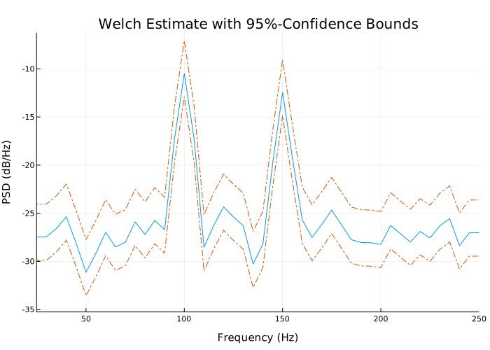
The power spectrum centered at zero frequency
Details
Let’s create a signal consisting of a sine wave with a frequency of 100 Hz in additive white noise . Reset the state of the random number generator to get reproducible results. The sampling rate is 1 kHz, the duration of the signal — 5 seconds.
using Random
Random.seed!(0)

Fs = 1000
t = 0:1/Fs:5-1/Fs

noisevar = 1/4
x = cos.(2π * 100 * t) + sqrt(noisevar) * randn(length(t))
We obtain a centered power spectrum using the Welch method using segments of length 500 counts, overlap 300 counts and DFT length 500 points.
import EngeeDSP.Functions: pwelch

pxx, f, pxxc = pwelch(x, 500, 300, 500, Fs, "centered", "power", out = :data)
Let’s plot the result graph. Power at frequencies −100 and 100 Hz is close to the expected power 1/4 for a real sine wave with amplitude 1. Deviation from 1/4 This is due to the influence of additive noise.
plot(f, 10 * log10.(pxx),
     xlabel = "Frequency (Hz)",
     ylabel = "Magnitude (dB)")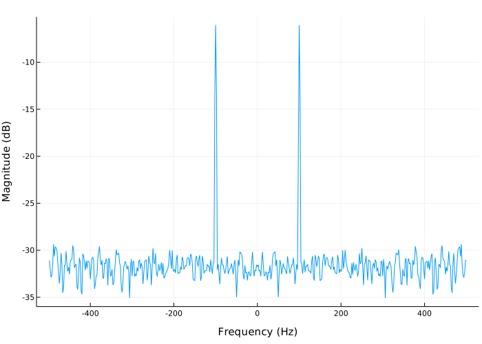
Evaluation of the SPM of a multichannel signal
Details
Generate 1024 sampling of a multi-channel signal consisting of three sinusoids with frequencies , and rad/counting in additive white Gaussian noise . Let’s evaluate Welch’s SPM and build a graph.
N = 1024
n = 0:N-1

w = π ./ [2, 3, 4]

using Random
Random.seed!(0)

x = cos.(w * collect(n)')' + randn(length(n), 3)

import EngeeDSP.Functions: pwelch

pwelch(x)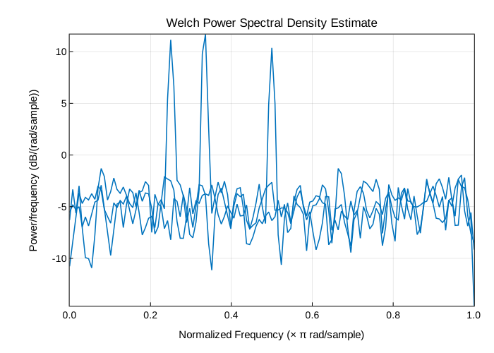
Additional Info
SPM estimation by averaging overlapping Welch segments
Details
The periodogram is not a consistent estimate of the true spectral power density of a stationary process in the broadest sense. The Welch method reduces the periodogram variance by splitting the input signal into overlapping segments.
The Welch method calculates a modified periodogram for each segment, and then averages these estimates to obtain an estimate of the spectral power density. Since the process is stationary in the broadest sense, and the Welch method uses estimates of the power spectral density of various segments of the input signal, the modified periodograms are approximately uncorrelated estimates of the true power spectral density, and averaging reduces variability.
Typically, the segments are multiplied by a window function, such as the Hamming window, so that the Welch method reduces to averaging modified periodograms. Because segments usually overlap, the data values at the beginning and end of the segment, smoothed by the window in one segment, are away from the ends of adjacent segments. This prevents information loss caused by using windowed mode.