Evaluation of amplifier parameters
Evaluation of amplifier parameters  — This is an Engee application designed to analyze the characteristics of power amplifiers (UM) based on measurement data, as well as build amp models with the possibility of using them in the Engee simulation environment. Signal analysis, model parameter setting, visualization of results, and export of coefficients for later use are supported.
To open the application, go to the Engee workspace and in the upper-left corner in the section Engee Applications ![]() choose Evaluation of amplifier parameters :
choose Evaluation of amplifier parameters :
Purpose and context of use
When transmitting a signal through power amplifiers (UM), especially in modes close to saturation, nonlinear distortions occur. This leads to two key effects:
-
Extending the signal spectrum beyond the bandwidth limits is a violation of the Spectral mask (ACLR) requirement;
-
In-band distortion and deterioration of transmission quality — increased power in adjacent channels (ACPR).
To increase the energy efficiency of transmitters, amplifiers often operate near saturation, where nonlinear effects occur. The problem is solved using the Digital signal pre-Distortion (DPD) method. The purpose of this method is to change (distort) the input signal in advance so that after passing through a real nonlinear MIND, the output signal is as close as possible to the ideal linear response. This allows you to:
-
Increase the efficiency of the amplifier;
-
Reduce non-linear distortion;
-
Reduce the level of inter-channel interference;
-
Ensure compliance with transmission standards.
The application supports several algorithms for adaptive tuning of the amplifier model:
-
RLS — recursive least squares method;
-
LMS — classical least squares method;
-
NLMS — normalized LMS;
-
RPEM — recursive error prediction method;
-
Regularized RLS is a modification of RLS with noise tolerance.
These methods allow you to dynamically adjust model parameters based on input and output signals.
Three model architectures are also supported:
| Architecture | Description |
|---|---|
P (Polynomial) |
The memory—free polynomial model is suitable for simple cases without pronounced hysteresis. |
MP (Memory Polynomial) |
Adds the effect of the "memory" of the amplifier, improves the accuracy of modeling time dependencies. |
GMP (Generalized Memory Polynomial) |
Extended architecture with additional cross members — used for complex distortions. |
The choice of a combination of algorithm and architecture affects the accuracy of the model. The evaluation criterion is usually the NMSE metric (normalized root-mean-square error).
Thus, the application Evaluation of amplifier parameters It allows you to model and adapt digital pre-image systems using both real and synthetic data.
Terms and abbreviations
-
DPD (Digital Pre-Distortion) — digital signal pre-distortion, a method for compensating nonlinear distortion of an amplifier.
-
NMSE (Normalized Mean Squared Error) is an indicator of the accuracy of the model, measured in decibels.
-
PAPR (Peak-to-Average Power Ratio) — the ratio of the peak value of the signal power to its average value.
-
ACLR (Adjacent Channel Leakage Ratio) — the radiation level in the adjacent frequency channel.
-
ACPR (Adjacent Channel Power Ratio) — the ratio of the power in the adjacent channel to the main one.
-
AM-AM is the dependence of the output amplitude on the input (amplitude-amplitude characteristic).
-
AM-PM is the dependence of the output phase on the input amplitude (amplitude-phase characteristic).
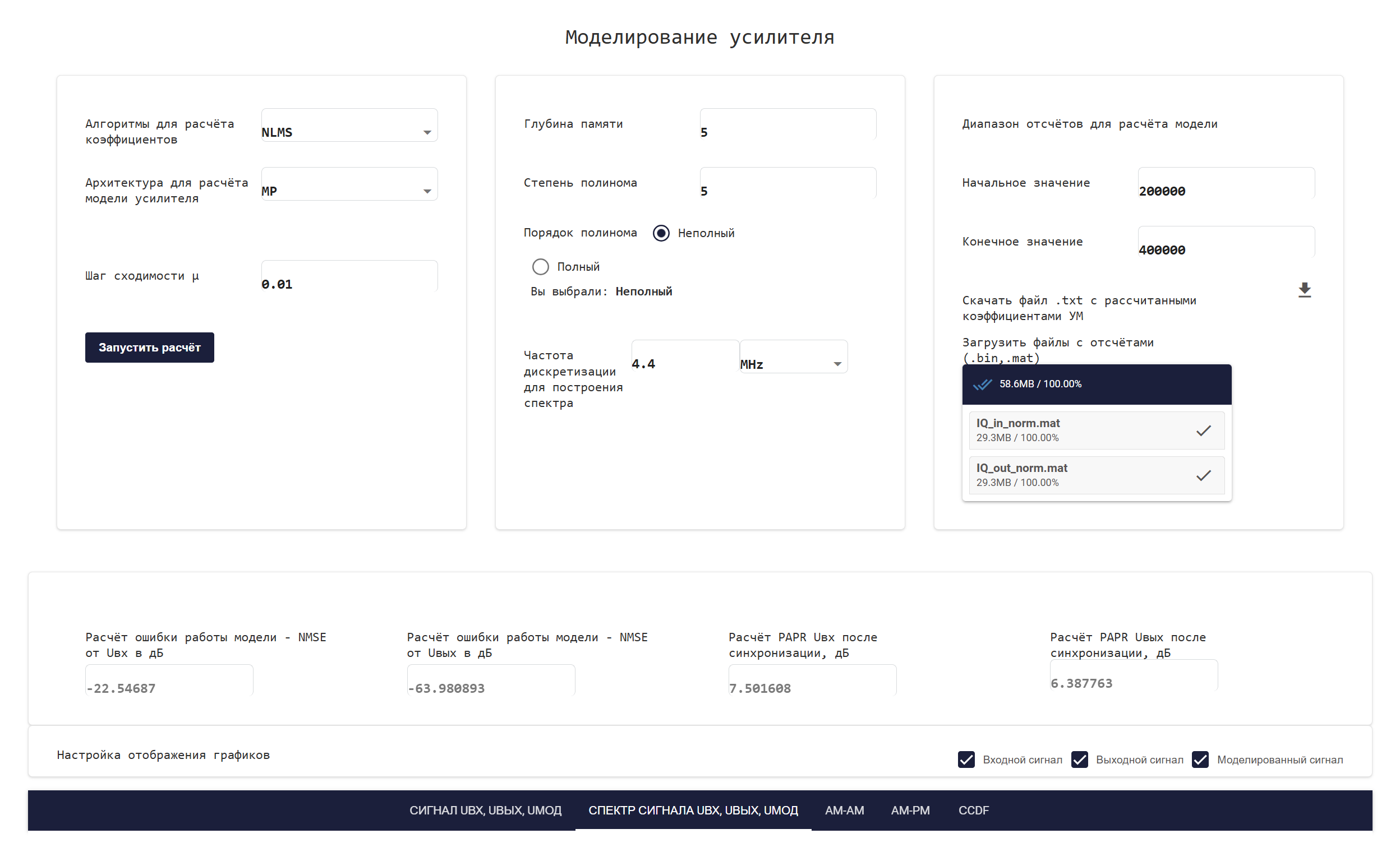
Application Interface
The application interface can be roughly divided into five sections:
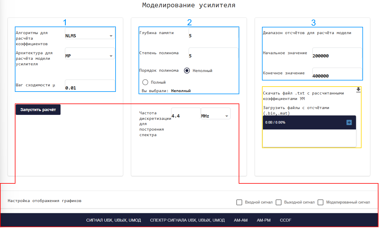
-
The yellow section is used for downloading files with amp counts and downloads.txt file with UM coefficients;
-
Three blue sections are used to adjust the amplifier model.;
-
The red section is the start of the model calculation, control of the sampling frequency of the spectrum signal for plotting, and the graph menu itself.
Next, let’s look at how to use the interface to consistently work with the application.
Working with the app
Loading input data
To get started, download two files with samples of the amplifier’s signals by clicking on the button  in the yellow section:
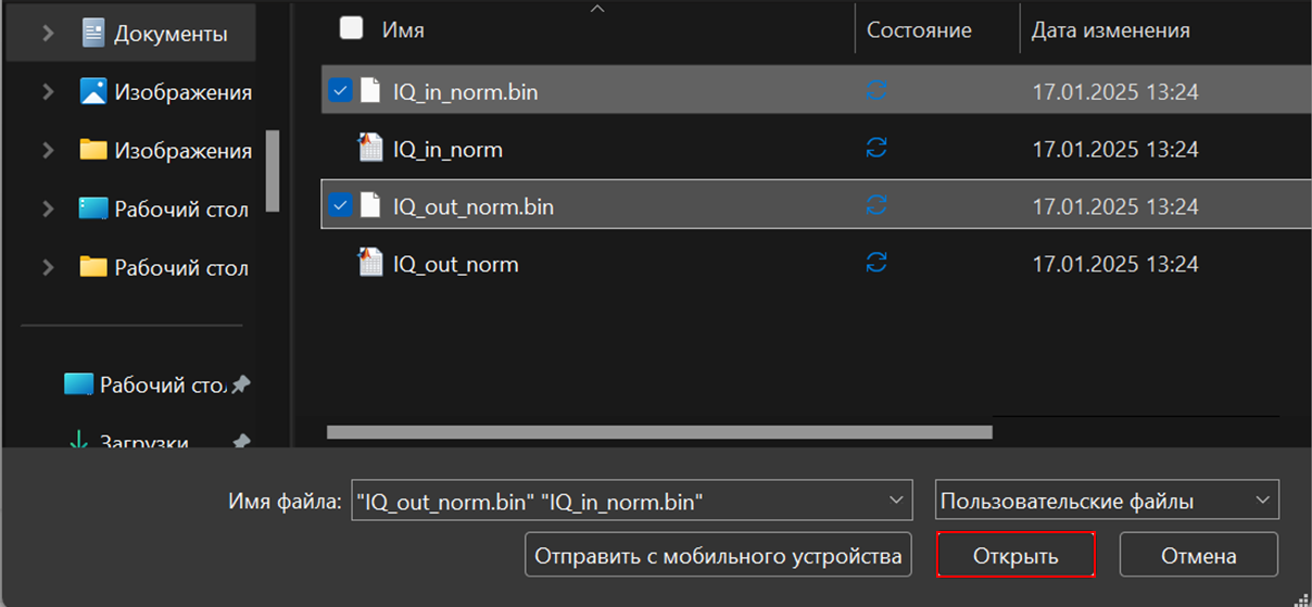
-
IQ_in_norm— signal samples at the input of the amplifier; -
IQ_out_norm— signal samples at the output of the amplifier.
|
The files with the counts must be named |
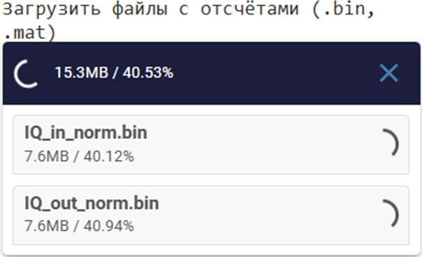
Files should be uploaded at the same time. To do this, select them via Ctrl+LKM in the window that opens:
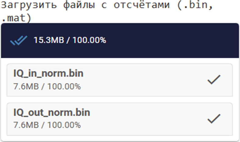
Wait for the files to download completely, the download indicators should change to ✓:
During the download process |
Done (✓) |
|---|---|
|
|
Setting up the amplifier model
Next, set up the model step by step in the blue sections:
-
Selection of algorithm and architecture (section No. 1) — the type of model and the DPD method (for example, NLMS) are set. Depending on the algorithm chosen, you will need to specify the convergence step or the degree of trust and the forgetting factor. No additional parameters are specified for the Moore-Penrose algorithm.
-
Model parameters (section No. 2) — the following parameters are set for models:
-
Memory depth;
-
Degree of the polynomial;
-
The order of the polynomial.
-
-
Sampling range (section No. 3) — indicates the range of samples used to calculate the model (by default: from
200000before400000).
Starting the model calculation
After setting up the amplifier model, start calculating it. To do this, click the Start calculation button. The indicator on the button will display the progress.
 →
→  →
→
After completion, the charting section will become available.
Plotting graphs
The following types of graphs are available:

-
Signals: input, output, simulated;
-
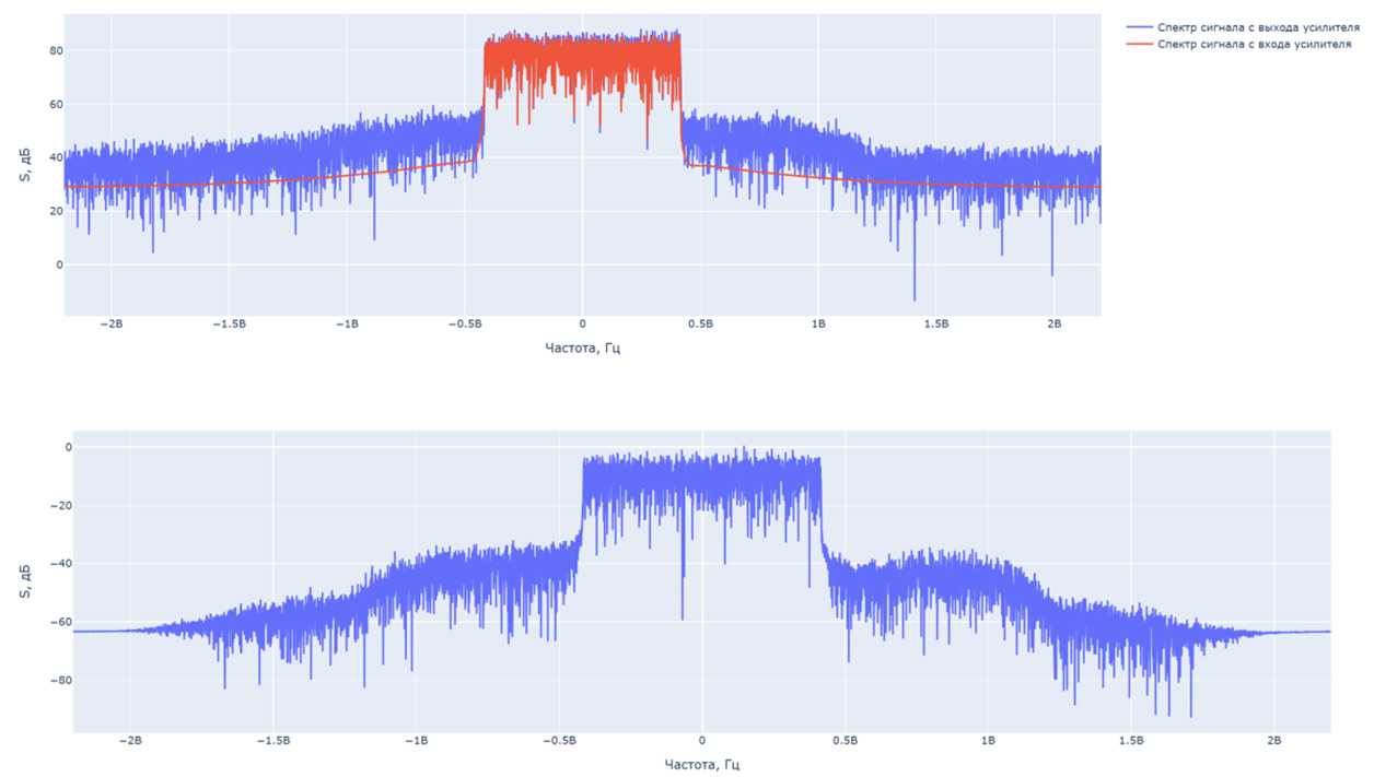
Signal spectra;
-
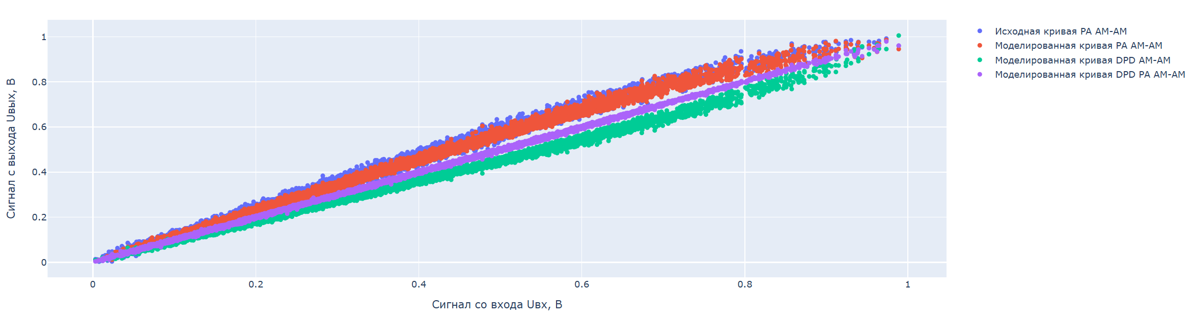
Characteristics of AM-AM and AM-PM;
-
Cumulative Distribution function (CCDF).
The sampling rate can be set manually.:

The classic functionality of the Plotly library will help you work with graphs more conveniently.:

-
 — download the graph as PNG.
 -
 — the ability to select an area and enlarge its contents.
 -
 — a tool for moving a graph on a coordinate plane.
 -
 — Zooms in on the coordinate plane.
 -
 — reduces the scale of the coordinate plane.
 -
 — returns the default scale of the coordinate plane.
 -
 — reset the coordinate axes.
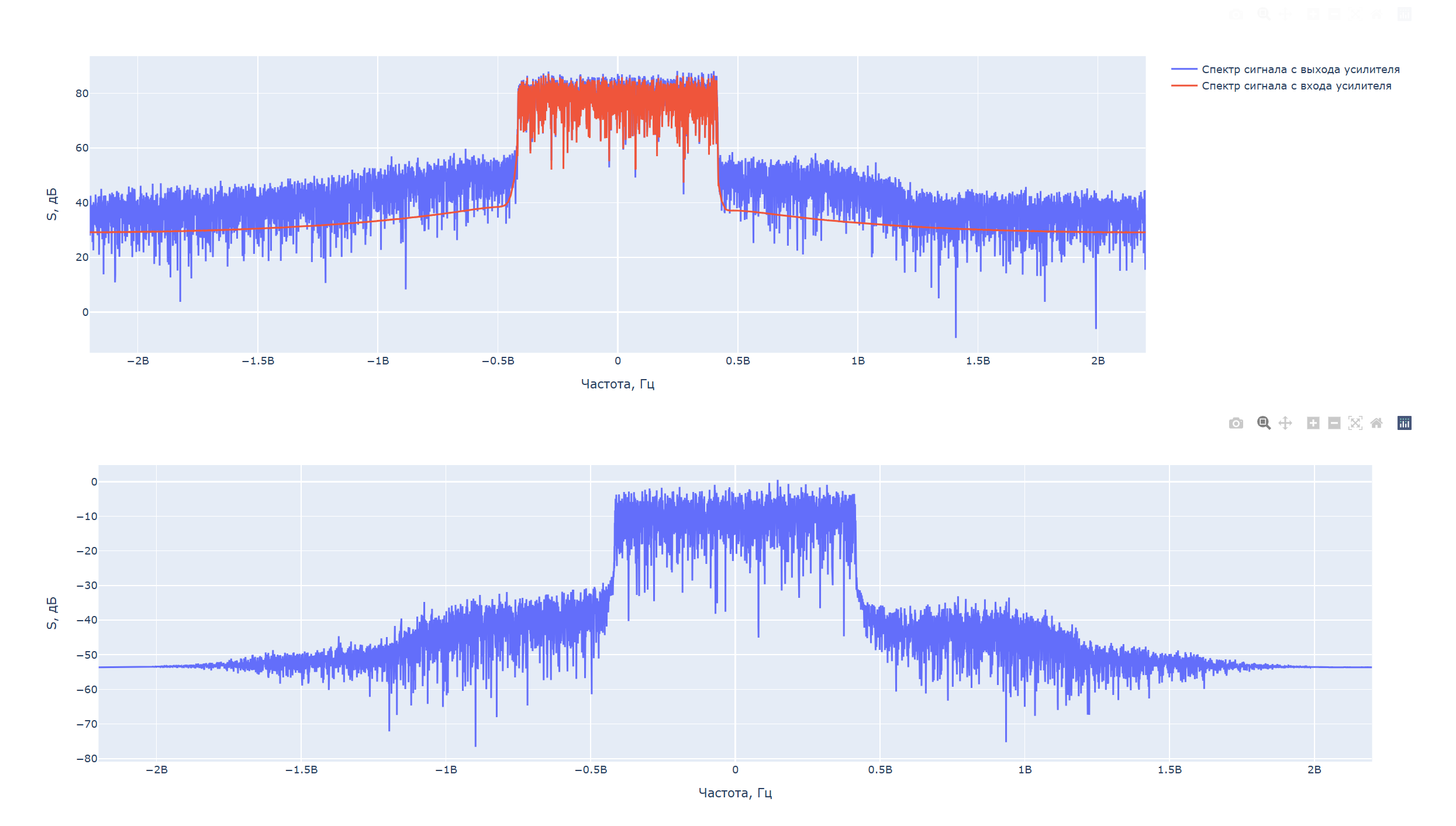
_ Examples of graphs_
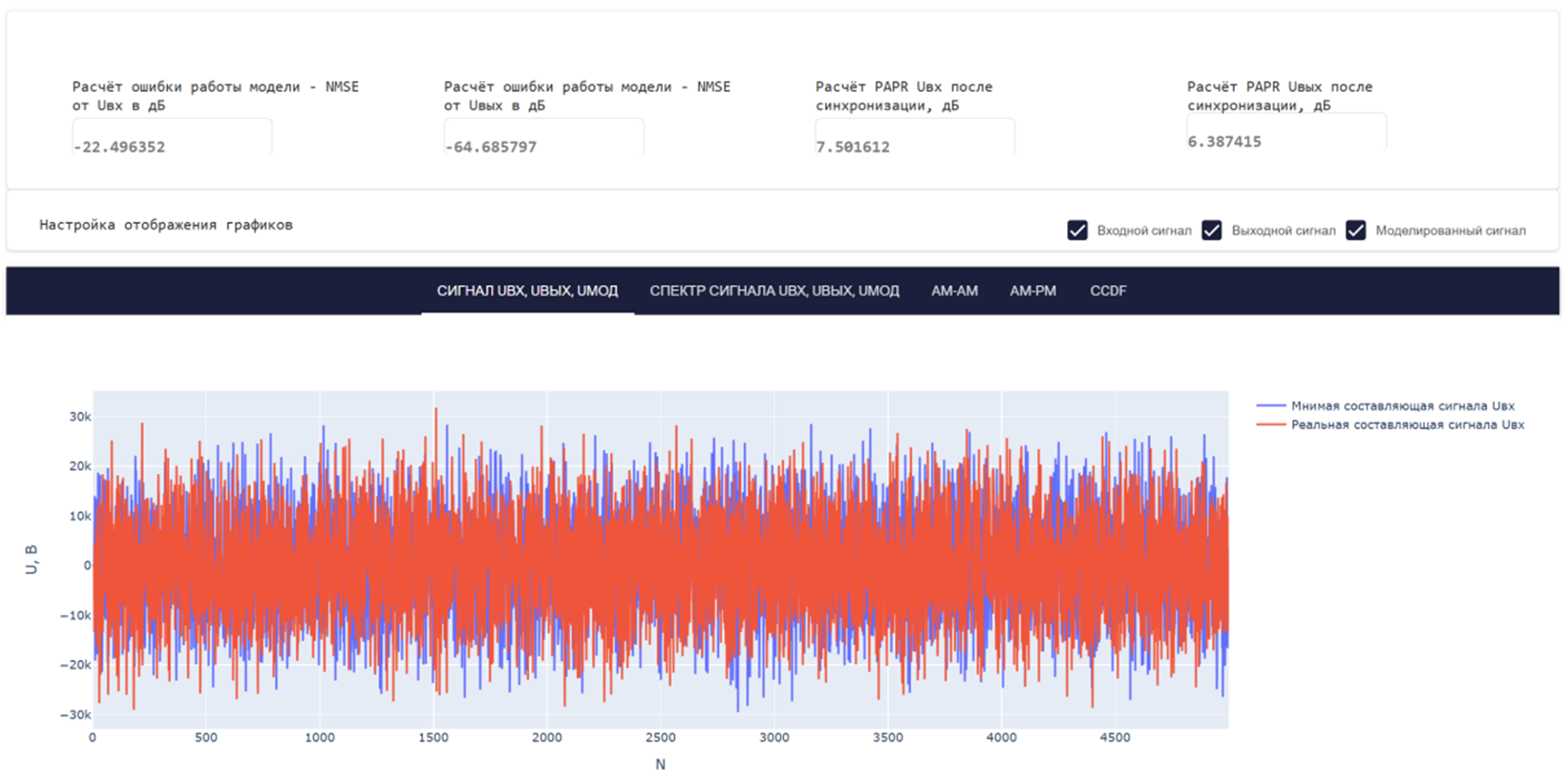
Signal spectrum Uinput, Uoutput, Umod:
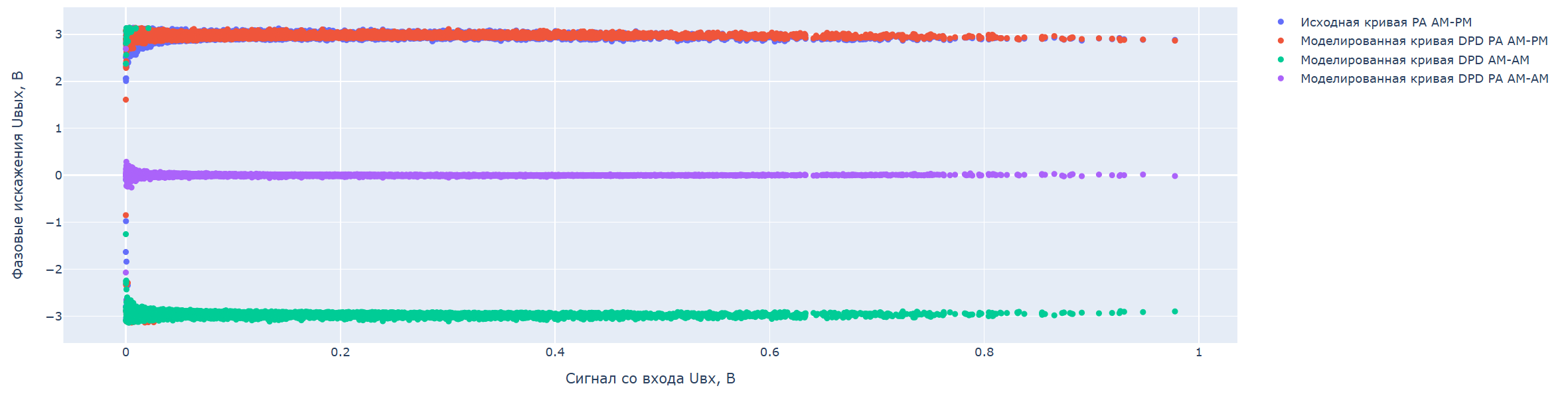
Amplitude-amplitude characteristic of AM-AM:
Amplitude-phase characteristic of AM-PM:
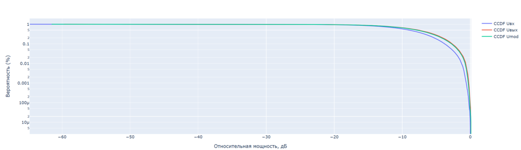
Cumulative probability distribution function CCDF:
To evaluate the efficiency of the amplifier model, the following are automatically calculated: normalized RMS error NMSE in dB, peak factor PAPR for the input, output and simulated signal, for example:
Loading coefficients
To save the coefficients of the model, click Download file. The file will be saved in the format .txt.