Data Inspector

Data inspector — this is an Engee application designed to work with the results of both one and several simulations, that is, a comparative analysis of the results of several model launches.

The application is used in two main scenarios:

Analysis of different signals of the same model, including comparative (comparison of different signals of the same model).
Comparative analysis of the results of different launches of the same model (comparing the same signal, but with different launches of the model).

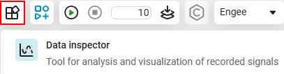
To open the application, go to the Engee workspace and in the upper-left corner in the section Engee applications choose Data inspector :

data inspector 1 en

Interface

The application works in a separate browser tab and by default looks like this:

data inspector 2 en

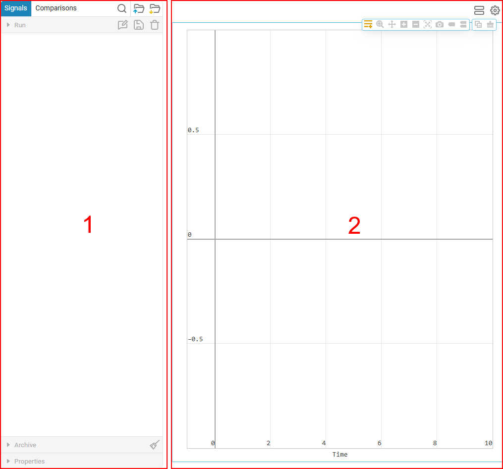
The window consists of two areas: signals (1) and graphs (2). Let’s look at them in more detail.

Signal area

The signal area contains all the signals from all runs of the model.

To analyze the signal after the simulation, you need to mark it as recordable before the model is launched. To do this, press the signal line and the button records signal logging 1 :

graph logging 1 en

Data inspector allows you to work with user sessions to simplify data analysis. A session is a set of parameters in the .ngdat format, which includes:

Window configuration signal visualization — saving the location of the axes, the number of rows and columns in the grid;
Displaying specific signals on selected axes, including the color scheme;
Saving current runs and their comparisons for further analysis.

Sessions can be saved and uploaded in the app.:

data inspector sessions en

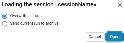
Loading the session — When loading a saved session, the data inspector completely restores the previously saved configuration.

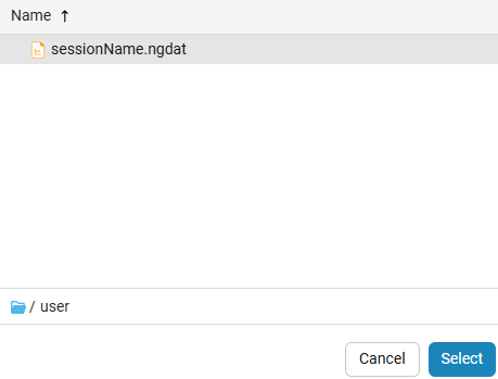
When loading the session, you can select:
- Completely clear the current runs and replace them with data from the downloaded session;
- Send the current run to the archive by making the run from the downloaded session active. Archived runs from the session are added to the shared archive.
Saving the session — This is the process of fixing the current configuration of the data inspector, including the settings of graphs, signals and runs.

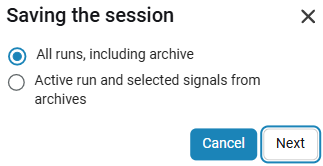
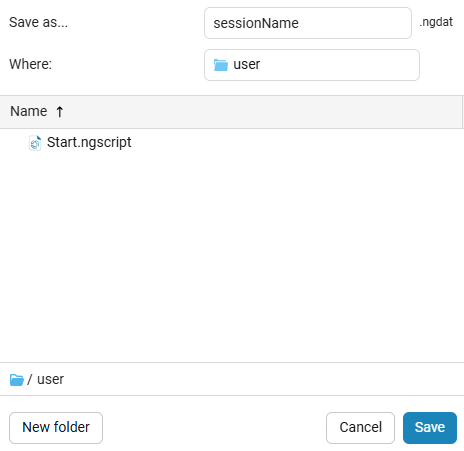
It is necessary to decide which runs to keep: All runs, including archive or Active run and selected signals from archives (marked with a check mark). By default, the session is saved in the /user directory with the name `sessionName'. Saved sessions will be available in file browser .

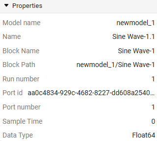
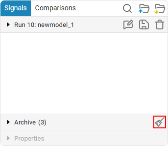
In the data inspector, the signals are grouped by runs.

data inspector 4 en

The active run is shown at the top of the signal area, all the others are collected below in the tab Archive. Clicking on the run name opens its properties window.:

data inspector settings 1 en

Options are available on the run panel:

Comment — here you can describe the features of a particular run, it will help when comparing with other runs.
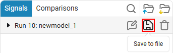
Save — all run signals can be saved to a CSV file.:
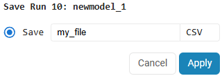
Delete — removing the run from the application.

You can delete all archived runs using the button Clear:

data inspector 5 en

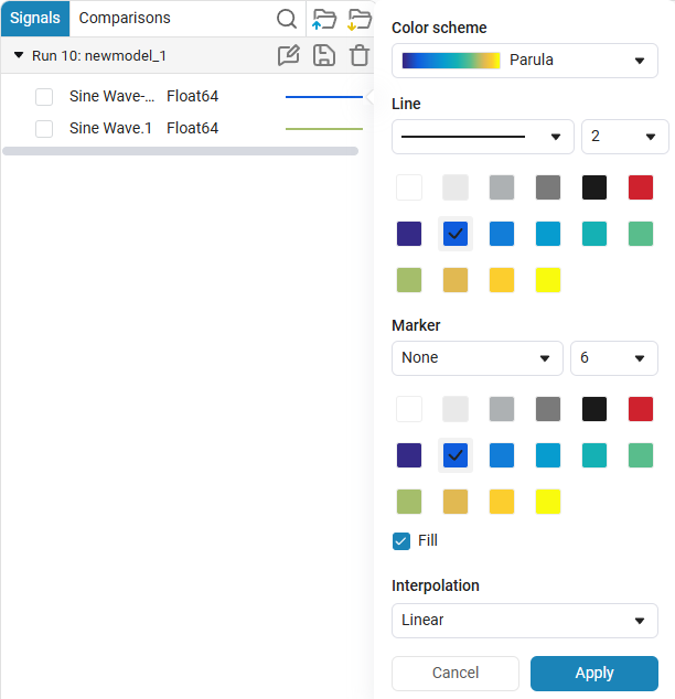
The color and line style can be changed for each signal. To do this, click on the colored stripe to the right of the signal name.:

data inspector 6 en

The checkbox to the left of the signal name is used to display the signal on the selected coordinate plane.

Chart area

The selected signals are displayed in the chart area. When you hover the mouse over the coordinate plane, a toolbar appears:

data inspector 7 en

Signal Menu — opens a menu with a choice of the type of signal display. Available time domain signals and dependence of one signal on another .
Zoom — performs scaling of the coordinate plane. It becomes possible to select an area and enlarge its contents. To return to the default scale, double-click on the coordinate plane with the left mouse button.
Pan — a tool for moving a graph on a coordinate plane. Allows you to move the chart in any direction using the mouse cursor.
Zoom in — Zooms in on the coordinate plane.
Zoom out — reduces the scale of the coordinate plane.
Autoscale — returns the default scale value of the coordinate plane.
Download plot as a png — Saves the coordinate plane to a PNG file.
One cursor — displays values on a graph when you hover the mouse pointer over it.
Two cursors — Displays values on all charts.
Copy to clipboard — copies the coordinate plane to the clipboard. You can insert a plane into Engee and other third-party programs.
Clear — removes the graph from the coordinate plane.

In addition to the main set of tools, there are two buttons available to you:

Axes arrangement — allows you to customize the graph output field. It offers a choice of chart layout templates from the basic presets or their self-configuration.:
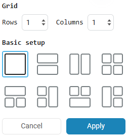
Settings — enables/disables the display of the legend of the name of the signals on the coordinate plane:

Storing/loading runs

The results obtained using the data inspector can be saved to a CSV file.:

data inspector wa 3 en

The file will be saved using the path `/user/run_data'. It is recommended to save the results of all important runs in order to be able to restore them if necessary. If the runs have been deleted from the archive or are not available for re-analysis in the inspector, they can be downloaded and played back using WorkspaceArray:

Use the function to clear the headers of the CSV file and the entry in the WorkspaceArray. The function will remove unnecessary prefixes, numbers, and spaces (the file header intended for export to WorkspaceArray should contain only the names of the columns time and `value' without spaces):

function clean_csv_header(file_path::String)
    # Reading lines from a csv file
    lines = readlines(file_path)

    # Splitting
headers = split(lines[1], ',')

    if length(headers) != 2
error("The file must contain exactly two columns.")
end

    # Header
processing time_header = "time" # adjusting the name of the first column, it should always be time
    value_header = strip(replace(split(headers[2], ".") |> last, r"\d+" => "")) # similarly for value

    # Create a new title bar
    cleaned_header = "$time_header,$value_header"

    # Overwriting a file
    open(file_path, "w") do file
        write(file, cleaned_header * "\n")
        write(file, join(lines[2:end], "\n"))
    end
end

file_path = "/user/run_data/my_file.csv" # path to the CSV file
clean_csv_header(file_path) # header cleanup

workspacecsv = WorkspaceArray("workspacearray_csv", "/user/run_data/my_file.csv") # write to WorkspaceArray

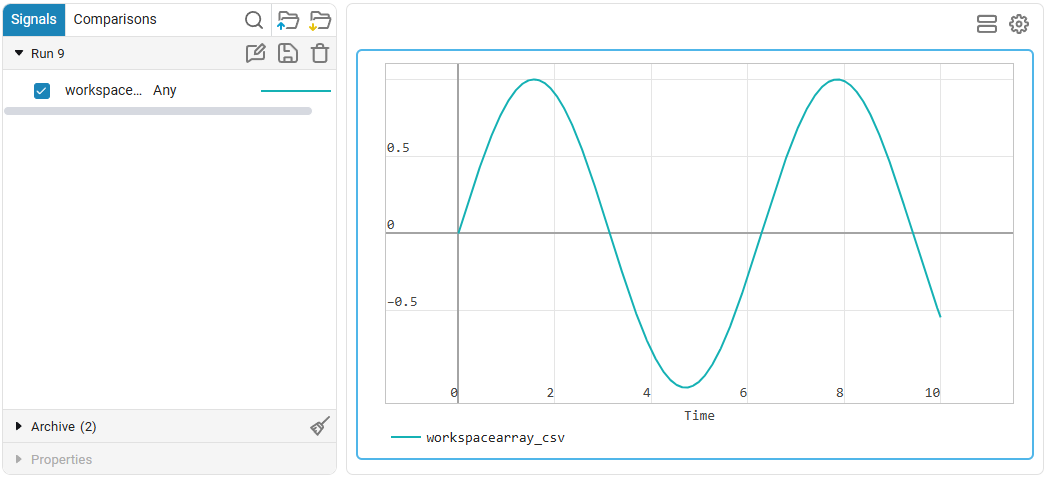
Open the data inspector, where the WorkspaceArray variable containing the simulation or run data will be displayed in the last run.:

Usage examples

Analyzing the results of a single simulation

Let’s take the following model as an example:

data inspector 8

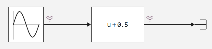
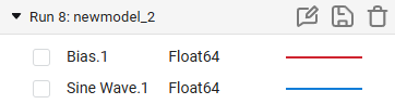
Block output signals Sine Wave and Bias marked as tracked. After the simulation of the model is completed, they can be seen in the Data Inspector:

data inspector 9 en

To add a signal graph to the coordinate plane, check the box next to the signal name.:

data inspector 11 en

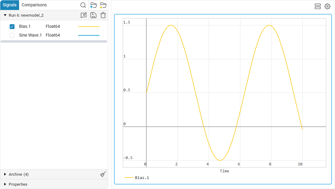
Optionally, you can configure the graph output field. Click the axis location button and choose a template with two smaller graphs on the left and one large one on the right.:

preset example 1 en

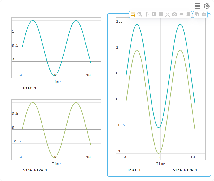
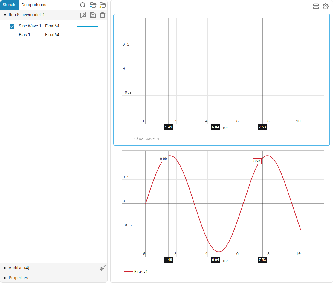
The values of the signals are visible when you hover the mouse over the graph. You can compare the signals on the same chart. For this:

Let’s check the boxes for those signals that we want to compare.
Enabling data comparison on hover .

When you hover the mouse, the values of both signals are displayed:

data inspector 12 en

Comparing multiple runs of a model

Data inspector allows you to compare several runs of a model with each other. This is useful, for example, to analyze the effect of a single parameter (or group of parameters) on the behavior of the model as a whole.

Changing the parameter value in the block Bias and let’s run the simulation. After the simulation is completed, a new run has become relevant in the application, and the previous one is available in the list "Archive»:

data inspector 13 en

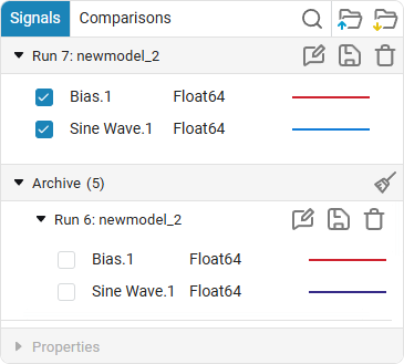
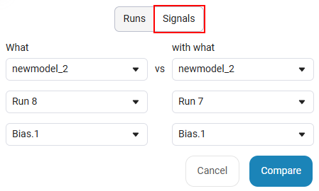
Let’s compare the runs and signals via the tab "Comparisons". Runs are compared within the same model:

data inspector run comparison en

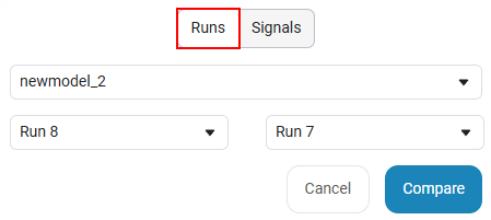
The signals can be compared from different models and runs.:

data inspector signals comparison en