Signal visualization
|
The window "Signal visualization" it is intended for visualization of model signals. To visualize graphs using code, use the tool Charts |
The window "Signal visualization» ![]() — one of the main visualization tools in Engee.
— one of the main visualization tools in Engee.
|
The window "Signal visualization»
|

Visualization of signals helps to understand and adjust the behavior of the model. Engee allows you to visualize signals as follows:
-
Basic:
-
Signal processing:
Signal Visualization Tools are used to work with graphs and coordinate planes.
Even more Engee visualization tools are presented in the Other Engee visualization Tools section.
The resulting graphs are easily exported (see Exporting a graph) in PNG or CSV format.
Use useful options to make it easier to work with the visualization window.:
-
Expand/compress charts horizontally and vertically:
-
Compress the coordinate plane vertically:
-
Hold down the name of the signal and move it to the graph (to set the name of the signal, double-click on it and enter the desired name):
-
Work with the signals of the same simulation on different coordinate planes. To do this, click Add chart
 and select the desired signal and the type of its display.
Time domain signals 
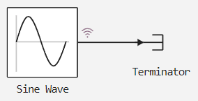
Create a model using blocks Sine Wave and Terminator, and turn on the recording  there are no signals between them. Leave all parameters and settings as default. The final model will look like this:
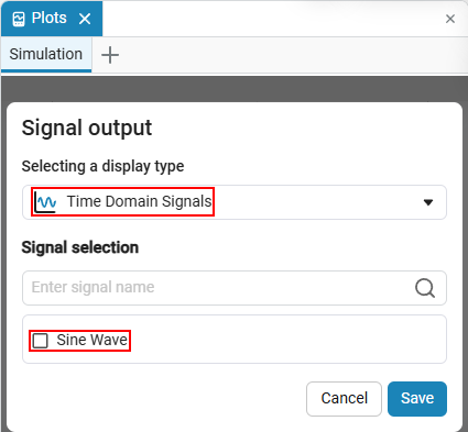
Start the simulation by clicking "Start»  . At the end of the simulation, to display the graph, click "Signal Menu»
  , select the display type and the signal is A sine wave generator:
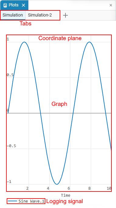
Now the graph of the sinusoidal signal simulation will be displayed in the visualization window. ![]() on the coordinate plane:
on the coordinate plane:
Signals in the frequency domain 
|
If the graph of the signal is in the frequency domain
The minimum required number of points is calculated based on Henning’s window function. To get the required number of points, you can either increase the Simulation time or decrease the Sample time. The formula applies to both Time-Based and Sample-Based blocks. |
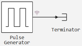
The frequency domain graph represents the spectrum of a signal, showing which frequencies are present in that signal. Create a model using blocks Pulse Generator and Terminator. Leave the default settings and enable recording. signals between blocks:
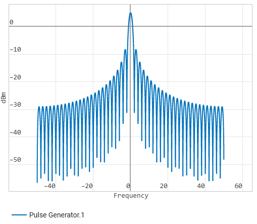
Set the simulation time to at least 16 seconds (otherwise there won’t be enough data points) and start the simulation with the button Start . After the simulation, open the visualization window ![]() and select the display type Frequency domain signals .
and select the display type Frequency domain signals .
After saving, you will receive the block’s signal spectrum. Pulse Generator:
|
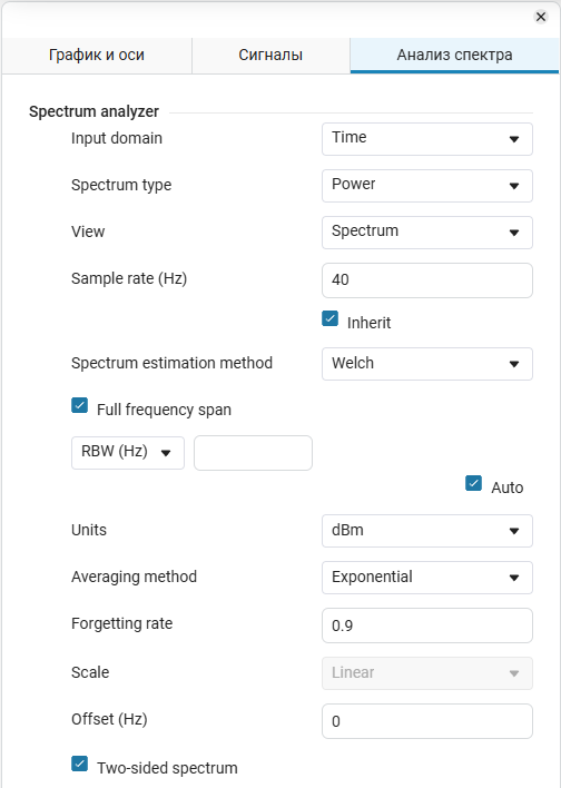
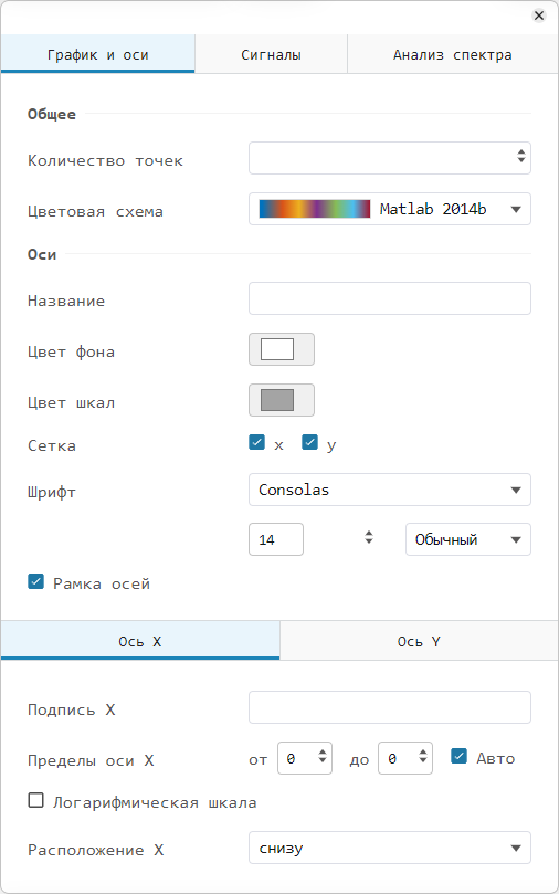
Additional settings of the model’s signal spectrum are available using spectrum analyzer graph windows. For this:
|

Dependence of one signal on another 
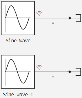
Create two models from blocks Sine Wave and Terminator, and turn on the recording there are no signals between them. Keep all the values of the block parameters and model settings by default, but increase the frequency for the Sine Wave-1 block (Frequency) with 1 before 2.
For clarity, specify a name for the signals by double—clicking on the signal from the block. Sine Wave and set the name to x, and for Sine Wave-1 set the name to y. The final model will look like this:
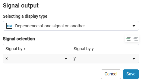
Start the simulation with the button Start . In the visualization window, select the display type. Dependence of one signal on another to open the signal selection window. Select x for the x-based signal and y for the y-based signal, respectively:
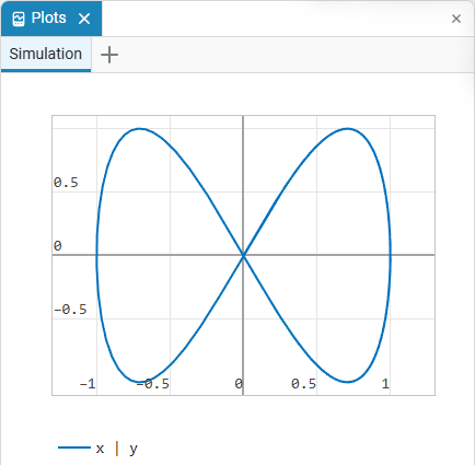
As a result, you will get the following graph (Lissajous figure):
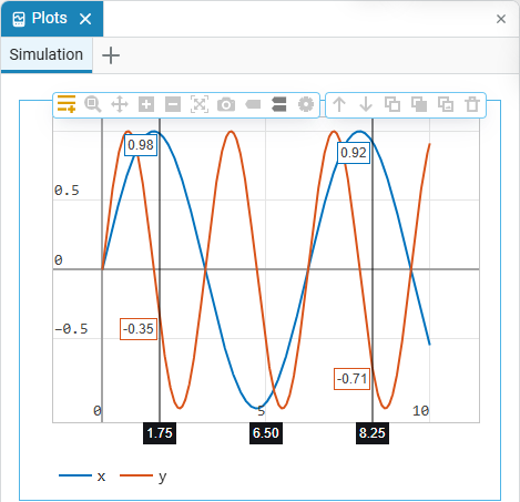
Graphs can also be compared in the time domain. . Use the same model. In the visualization window, use the button Signal Menu switch to Time Domain Signals and select both signals.
Next, hover the cursor over the coordinate plane, select Two cursors  in the tools menu. Select the desired point on the chart and compare the values of the signals with each other:
Signals in tabular form 
Assemble the following model from blocks Sine Wave, Constant, Identity Matrix and Terminator:
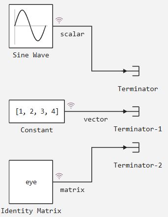
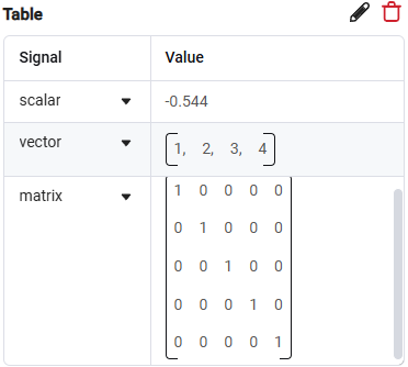
For the block Constant set the value [1, 2, 3, 4]. Next, start the simulation with the button Start . After the simulation, select the type in the visualization window Signals in tabular form to open a table with instantaneous signal values:
To switch to other display types, use  .
.
A frame in the time domain 
Time domain frame ![]() — the model processes multiple data elements in one time step. Read more about frame-by-frame signal processing in Engee in the article Signal processing by frames and counts.
— the model processes multiple data elements in one time step. Read more about frame-by-frame signal processing in Engee in the article Signal processing by frames and counts.
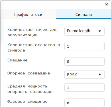
The signal constellation 
Constellation diagram A constellation diagram is a graphical method of representing modulated signals in digital communications. It is used to visualize the symbols transmitted in a modulated signal, and helps analyze the quality of data transmission and detect distortions. Read more in the article Signal constellations.
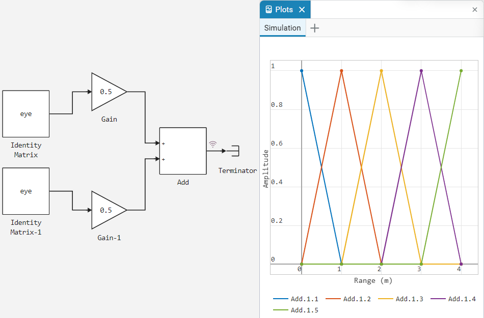
Building an array 
Array plot ![]() — this is the process of graphical visualization of data organized into arrays. It allows you to interpret numerical data as functions of time or other variables, displaying them as continuous lines and points.:
— this is the process of graphical visualization of data organized into arrays. It allows you to interpret numerical data as functions of time or other variables, displaying them as continuous lines and points.:
Eye diagram 
Eye diagram — It is a tool for analyzing digital signals, which helps to identify errors and distortions in data transmission. It displays repeatedly superimposed time sections of the signal, creating an image resembling an eye. This allows you to visually see signal distortions such as: intersymbol interference (ISI), noise, duty cycle distortion, and other interference.
An important advantage of the eye diagram is the ability to evaluate the quality of data transmission by the width and shape of the "eye" — the more open the "eye", the better the signal transmission.
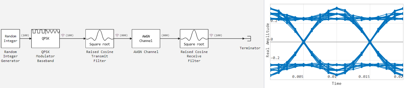
The diagram is used to analyze noisy signals in order to understand how well data is transmitted over the communication channel. For example, an eye diagram helps to identify deviations from an ideal signal caused by factors such as frequency offsets or phase errors.
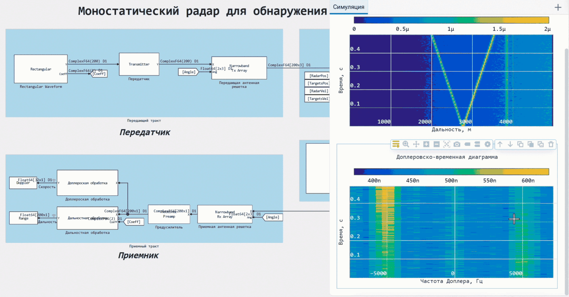
Intensity chart 
Intensity Scope — It is a visualization tool that is used to display the power distribution or amplitude of a signal depending on coordinates or time parameters. It helps to analyze changes in signal intensity at different points in space or in time, which is especially useful in radar and digital signal processing (DSP).
The intensity diagram allows you to visually assess how the signal energy is distributed in the study area. For example, in optical systems, it helps to analyze the distribution of light in a beam, to identify the focusing and divergence of rays. In radio engineering and acoustics, it is used to study radiation patterns and signal levels in various directions.
Signal Visualization Tools
Depending on the choice of the type of signal display, different graphs are obtained that are useful for individual situations. But this is only part of the functionality of the window "Signal visualizationNext, let’s look at the toolbar and its features.
To view the available visualization window tools ![]() move the mouse cursor over the coordinate plane. There are two sets of tools available in total:
move the mouse cursor over the coordinate plane. There are two sets of tools available in total:
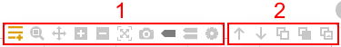
_ Overview of the Signal Visualization window tools_
The first set |
The second set |
||
The first set contains everything you need to work with graphs.:
|
The second set is designed to work with two or more coordinate planes.:
|


To add a new coordinate plane, use the button . This button will allow you to adjust the plane before adding it and will re-display the menu for displaying signals and display types. The new plane will be added above the old one by default. You can change their order using the tools.
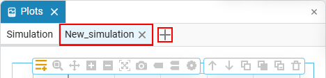
To add a new tab in the visualization window, use the button New tab  and give her a name. In the created tab, you can work with new or existing simulation results in the usual mode.
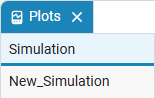
For convenience, the tabs can be positioned vertically.:
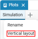 →
→ 
Exporting a graph
- There are three ways to export a chart
-
-
Save the coordinate plane as an image using the button Download plot as a png
 . The image will be automatically uploaded to your computer using the path specified in your operating system.
 -
Insert the image of the coordinate plane into Engee and into third-party programs using the button Copy to clipboard
 .
. -
You cannot export the graph to CSV directly, but you can export its signal data using the block To CSV. To do this, set up a block To CSV to output the desired model signal and in the parameter File name In the block, specify the name of the future CSV file (untitled.csv by default). The CSV file will be saved in file browser Engee under the specified name.
-
Other Engee visualization Tools
If your visualization tasks are much broader than described in the previous sections, then Engee offers you other tools. Review them to choose the best solution for visualizing the results of your models.:
-
Data Inspector allows you to view, analyze and compare the results of both one and several simulations (runs).
-
The simout variable allows you to work with the simulation results of the model via the command line or script editor, for example, using the library Plots.