Spectrum Analyzer
Spectrum analyzer is a tool for analyzing the frequency composition of a signal. The operation of the spectrum analyzer is based on the method fast Fourier transform.
To configure the spectrum analyzer:
-
Open Signal visualization
 .
. -
Select the type of signal display Frequency domain signals
 using the button Signal Menu
  .
. -
In tools click on the button Settings
 and go to the section Spectrum analyzer.
Spectrum Analyzer Interface
The interface of the spectrum analyzer consists of the following settings:
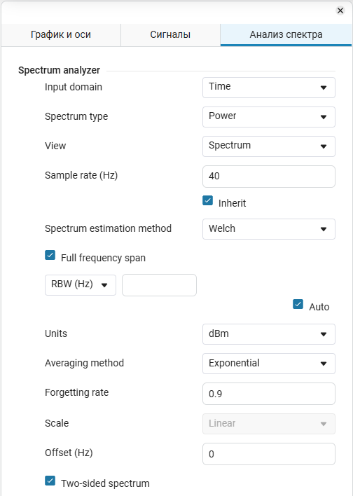
Input domain — working with the time domain of the signal
+
Time
Details
The input signal that you supply to the spectrum analyzer is represented as a time sequence, and the spectrum will be analyzed in the context of that time.
Spectrum type — type of spectral analysis
+
Power (by default) | Power density
Details
Indicates the type of spectral analysis. It has two meanings — Power and Power density. Both values affect the parameter setting. Units:
-
Power density— divides the value of the spectrum module by the frequency, allows you to analyze the spectrum in the frequency range:.
-
Power— leaves the values of the spectrum modulus unchanged (removes division), allows you to analyze the signal spectrum by amplitude:.
View — type of presentation of the results of the signal spectrum analysis
+
Spectrum (by default)
Details
The view can be represented using a single parameter. — Spectrum. This means that you will receive the results of the analysis in the form of a signal spectrum. Presented with only one option.
Sample rate (Hz) — the rate of measurement or sampling of the signal in time
+
100 (default)
Details
The setting indicates the number of signal samples recorded within one second. It is set as a positive scalar number.
Dependencies
-
If the parameter is checked Inherit enabled (by default), the sampling rate will be automatically determined based on the characteristics of the input signal. In this case, the spectral analysis will be performed taking into account the automatically determined sampling frequency.
-
If the parameter is checked Inherit turned off, the sampling frequency of the signal will be set to a certain value specified in the parameter Sample rate (Hz). This means that the spectral analysis will be performed taking into account the given sampling frequency, and the analysis results will be displayed for this frequency.
Spectrum estimation method — the method of spectrum analysis
+
Welch (by default)
Details
Engee uses the method of spectral analysis Welch. For more information, see The Welch method. Presented with only one option.
Full frequency span — the ability to set frequency values
+
Enabled (by default) | Turned off
Details
The parameter determines whether the entire available frequency range in the signal will be analyzed or whether only a specific range will be used.
-
Enabled (by default)— The spectrum analyzer will cover all the frequencies available in the signal from0(minimum) to infinity (maximum). -
Turned off— The spectrum analyzer will cover only the manually set range.
Dependencies
To enable the parameters FStop (Hz) and Span (Hz) remove the flag Full frequency span.
FStart (Hz) —
the initial value of the frequency coverage
range
Not set (by default)
Details
This parameter allows you to manually determine the set value of the frequency coverage range (at the beginning of the range). It is set as a positive scalar number.
Dependencies
When selecting an option FStart (Hz) the parameter is added automatically FStop (Hz).
FStop (Hz) —
the final value of the frequency coverage
range
Not set (by default)
Details
The parameter allows you to manually determine the set value of the frequency coverage range (at the end of the range). It is set as a positive scalar number.
Span (Hz) — range of values around the central frequency
+
Not set (by default)
Details
It is used to set the range of analysis values around a point (center frequency) on the frequency axis.
Dependencies
When selecting an option Span (Hz) the parameter is added automatically CF (Hz) (central frequency).
CF (Hz) — central frequency
+
0 (default)
Details
The central frequency around which the signal is processed as a positive scalar number.
By default, the spectrum analyzer sets CF (Hz) in the middle of the range to ensure uniform frequency coverage.
RBW (Hz) — frequency resolution
+
Not set (by default)
Details
The parameter indicates the frequency resolution of the displayed spectrum and determines with what accuracy we can display the frequency components of the signal during analysis. The lower the value is RBW (Hz) the higher the resolution of the spectrum analyzer, but also the more signal samples (simulation time) are required for measurements.
|
Parameter RBW (Hz) it directly affects the display of the signal in the frequency domain:
|
Units — selection of measurement units for the amplitude of the spectral components of the signal
+
dBm (by default) | dBW | Watts
Details
The parameter defines the units of measurement for the amplitude of the spectral components of the signal in decibels milliwatts (dBm), decibels of watts (dBW) and watts (Watts).
Averaging method — choice of the spectrum averaging method
+
Exponential (by default) | Running
Details
The parameter defines the averaging method used to reduce noise and variations in the spectrum data, which makes the spectrum smoother and more suitable for analyzing stationary signal components. There are two methods available:
-
Exponential— uses a weighted average of the current and previous values of the signal spectrum samples. The weight of the previous spectrum values decreases exponentially with the "forgetting" coefficient, which is set in the parameter value field. Forgetting rate. -
Running— uses the working average of the latest samples to smooth the data.
Forgetting rate — numerical input of the sample weight
+
0.9 (default)
Details
Numerical input of the sample weight from 0 before 1.
Dependencies
To use this parameter, set for the parameter Averaging method meaning Exponential.
Scale — display of frequency values on the axes of the spectrum graph
+
Linear (by default) | Log
Details
There are two options for displaying the scale:
-
Linear— the frequencies are evenly distributed with a constant step between each point. This means that each interval on the frequency axis has the same length and changes in frequency are displayed proportionally on the graph. -
Log— the frequencies increase in accordance with the logarithmic function, which leads to a uniform distribution of values on the axis in the case of exponential growth or decrease.
independency
Enabling the checkbox Two-sided spectrum blocks the use of the parameter Scale.
Offset (Hz) — determines the value of the constant component of the signal, shifting along the frequency axis on the spectral graph
+
0 (default)
Details
Parameter Offset (Hz) indicates the frequency by which the signal is shifted in the spectral representation. For example, if the constant offset frequency is 100 Hz, then the entire spectrum will be shifted to 100 Hz to the right or left relative to the zero frequency. By default, the spectrum will not be shifted.
Two-sided spectrum — a method for visualizing the signal spectrum, which displays both positive and negative frequencies
+
Enabled (by default) | Turned off
Details
When the parameter is enabled, the frequency axis is centered around zero and both positive (double) and negative (decrease by two) frequency values are displayed on the graph. This allows you to simultaneously see both the amplitude characteristics of the signal at both positive and negative frequencies.
Example
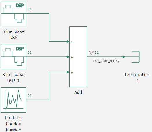
Let’s look at the principle of operation of a spectrum analyzer using an example. To do this, we will build a model from two blocks of sinusoid sources. DSP Sine Wave from the digital signal processing library and the pseudo-random sequence source (noise source) block Uniform Random Number. We will complete the model using the input signal addition or subtraction block. Add and stubs for the output port Terminator. As a result, we get the following model:
Let’s change the settings of the blocks and the solver:
Sine Wave DSP |
Amplitude = |
|---|---|
Sine Wave DSP-1 |
Amplitude = |
Uniform Random Number |
Minimum = |
Add |
List of signs = Quantity |
Solver |
Step Size = |
Turn it on signal recording  from the block Add. (for convenience, give a name
 Two_sine_noisy) and start the simulation of the model with the button Start  .
.
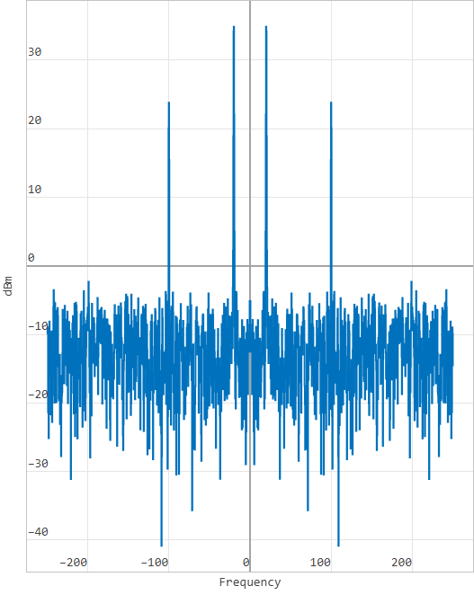
Open Signal visualization ![]() . By default, the time domain graph is displayed on the coordinate plane. To view the graph in the frequency domain, select the display type Frequency domain signals in Signal Menu on toolbars chart windows and check the box to display the signal
. By default, the time domain graph is displayed on the coordinate plane. To view the graph in the frequency domain, select the display type Frequency domain signals in Signal Menu on toolbars chart windows and check the box to display the signal Two_sine_noisy:
Go to the spectrum analyzer settings using the Settings button and select the tab Spectrum analyzer. To display the graph in the frequency domain, it is important to take into account the frequency resolution parameter. RBW (Hz):
-
If the parameter has RBW (Hz) if the value is automatically determined, then the graph in the frequency domain will be displayed if the condition is met:
,
where 1536 is the minimum number of data points required to plot a graph in the frequency domain, obtained from Henning’s window function. To get the minimum number of points, either increase
Simulation time(simulation time), or reduceSample time(calculation step). The formula applies to both Time Based and Sample Based blocks.For example, for the current model, you need at least
3.2seconds of simulation, because satisfies the condition. -
If the parameter has RBW (Hz) If there is a specific value, the graph will be displayed if the condition is met:
,
where — the minimum required number of points; — a constant that depends on the selected window function. In Engee, this is a Henning window function, so the value of the constant is
1.5. — sampling rate.For example, for the current model Hz, Hz, . Let’s substitute the values in the upper expression and see what is needed at least
750points for plotting. Behind1The model gets a second of simulation.500data points, therefore, at least1.5seconds of simulation.
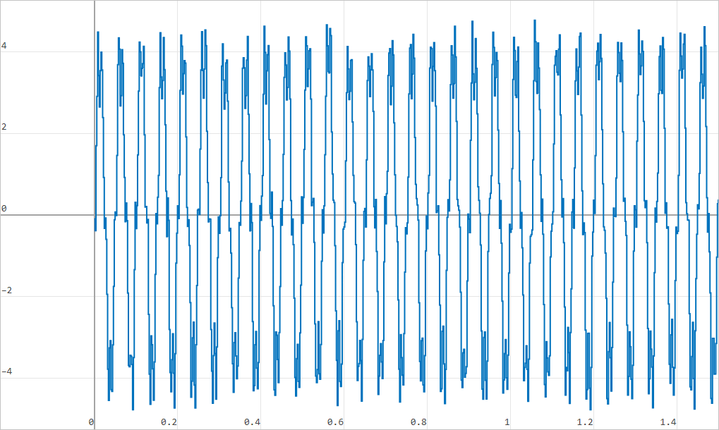
To view the graph in the time domain, select the display type Time Domain Signals  in Signal Menu and check the box to display the signal
 Two_sine_noisy:
The Welch method
Engee uses the Welch method to operate the spectrum analyzer.
The Welch method is a spectral analysis method that is used to estimate the power spectrum of a signal. It is a modification of the Fourier transform and makes it possible to improve the statistical properties of the spectrum estimation by dividing the signal into overlapping segments and averaging their spectral estimates.
The description of the method’s operation
When choosing the Welch method, the power spectrum estimate is an averaged modified periodogram. The algorithm in the spectrum analyzer consists of the following steps:
-
The block buffers the input signal into data segments by points. Each data segment is divided into overlapping data segments, each with a length of , overlapping on points. The data segments can be represented as:
-
If , then the overlap is 50%.
-
If , then the overlap is 0%.
-
-
Apply a window to each of the overlapping data segments in the time domain.
If for the parameter Full frequency span If the checkbox is unchecked, you can set the length of the data window. using the parameter Span (Hz) or using the parameters FStart (Hz) and FStop (Hz).
If you have set for the parameter Full frequency span meaning the algorithm determines the length of the data window using this equation:
.
It then splits the input signal into several data segments with a window.
Most window functions have a greater impact on the data in the center of the set than on the data at the edges, which represents a loss of information. To mitigate this loss, the individual data sets usually overlap in time. For each segment with a window, calculate the periodogram using the discrete Fourier transform. Then calculate the square of the result value and divide it by :
where U is the power normalization coefficient in the window function, which is defined as follows:
.
-
The spectrum analyzer calculates and plots the power spectrum, power spectral density, and RMS value using a modified periodogram estimation method.
To determine the Welch power spectrum estimate, the spectrum analyzer averages the periodogram results for the latter data segments. Averaging reduces the variance compared to the original data segment from points.
here:
-
The spectrum analyzer calculates the spectral power density using:
-
The power spectrum is the product of the power spectral density and the resolution bandwidth, as shown in this equation:
-
In the mode Spectrum The spectrum analyzer plots the power graph as a spectrogram. Each line of the spectrogram is one periodogram. The time resolution of each row is , which is the minimum achievable resolution. To achieve the desired resolution, it may be necessary to combine several periodograms. To calculate non-integer values interpolation is used. On the spectrogram display, time scrolls from top to bottom, so the most recent data is displayed at the top of the display. The offset shows the time value at which the center of the most recent line of the spectrogram is located.
-
The spectrum analyzer requires a minimum number of samples to calculate the spectral estimate. This value is directly related to the resolution band ( ) using this equation:
or the length of the window ( ) using the equation:
,
where — percentage of overlap, — normalized effective noise band, — the frequency of the input sample, — resolution band.
The spectrum analyzer shows the number of samples per update in the status bar of the spectrum analyzer. If the resolution method is set to , then the window length is determined by:
.