Settings
Settings Window ![]() — An Engee tool designed for configuring blocks, models, and simulations.
— An Engee tool designed for configuring blocks, models, and simulations.
To open the model and simulation settings window, click on the gear icon. ![]() in the workspace of the model.
in the workspace of the model.
The settings window consists of three tabs:
and other tabs if the block settings are selected.
To switch between the settings tabs, click on their titles or hover over the status bar.:
![]()
To access the block settings, double-click on the block icon or click once on the block with the settings window already open.:
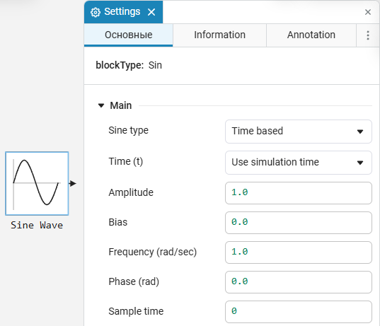
Block Parameters
The tabs of the settings window for the blocks differ depending on the selected block. By default, each block has two main tabs — Main and a tab Information:
-
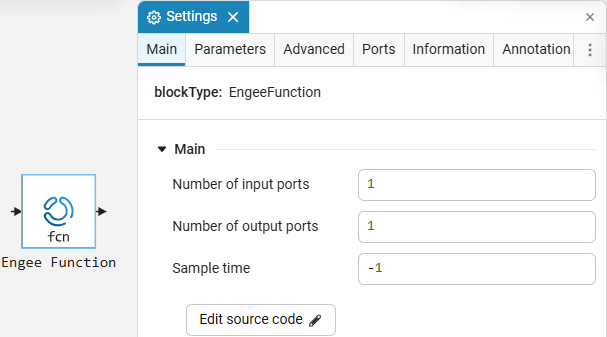
The Basic tab specifies the block parameters, as well as other special settings that allow you to control its behavior. For example, for Engee Function this is an opportunity to edit the source code of the block.:
Block parameters can be set using expressions (for more information, see here). -
On the tab Information useful information about the selected block is provided. The block name can be changed via this tab. Click the button
 to go to the reference documentation for the selected block.
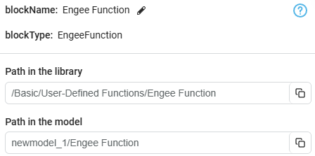
The "Properties" tab
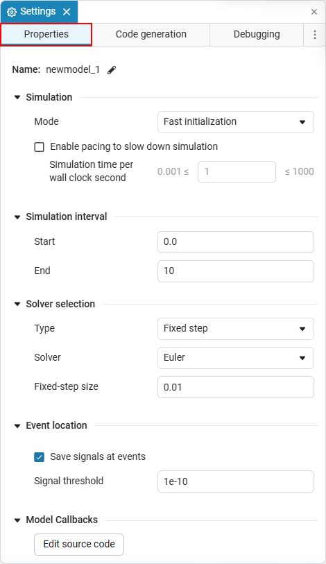
This tab is used to configure the main parameters of the model in Engee. The options are available in the tab solvers, event detection and management callbacks. These options allow you to influence the calculation of the model, control the model’s response to events, and use your own functions to expand modeling capabilities.
So, the tab consists of the following fields:
-
Name — displays the name of the current model (newmodel_1 by default).
-
Mode — defines a simulation execution method that balances between the initialization speed of the model and the calculation speed. There are two modes available:
-
Fast initialization — the mode in which the model starts as quickly as possible due to simplified typing and disabling optimizations. It is suitable for debugging large models when it is necessary to minimize the simulation startup time, for example, with frequent changes in the model structure.;
-
Fast simulation — a mode designed to maximize the reduction of computing time by performing deeper code optimization and a high degree of specialization of computational algorithms. It is most suitable for performing final calculations or simulations where high performance and minimal calculation time are important.
-
-
Enable pacing to slow down simulation — indicates how many seconds of the simulation should be completed in a real second. Use this setting to slow down the simulation and simplify the analysis and interaction with the model.
-
Start — the initial simulation time (by default
0.0). -
End — the end time of the simulation (by default
10). -
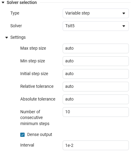
Type — type selection solver (Fixed step / Variable step):
Fixed step Variable step 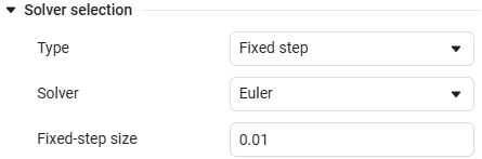
-
Solver — solver selection (default is Euler).
-
Fixed-step size — the value of the integration step (by default
0.01).
-
Max step size — setting the maximum integration step (by default
auto). -
Min step size — setting the minimum integration step (by default
auto). -
Initial step size — setting the initial integration step (by default
auto). -
Relative tolerance — setting the relative accuracy of integration (by default
auto). -
Absolute tolerance — setting the absolute accuracy of integration (by default
auto). -
Dense output — enables/disables the dense output function. If this option is selected, Engee will output results with a higher frequency (enabled by default).
-
Interval — the interval at which dense output occurs (by default
1e-2).
-
-
Save signals at events — Saves signals at the time of event detection (enabled by default).
-
Signal threshold — the threshold of the signal that is used to detect events (by default
1e-10). -
Edit source code — opening the callback source code editor. This option is intended for more advanced control over the behavior of the model.
Tab "Code generation»
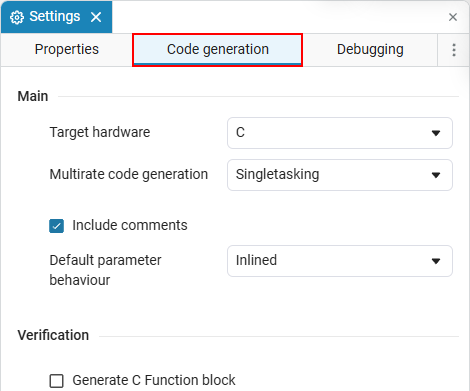
About the functions of the tab Code generation read in the article Code Generator Features.
More information about code generation in Engee can be found in the series of articles. Code generation.
Tab "Debugging»
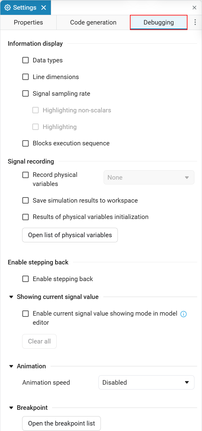
- You can use this tab to display information about the model and save the simulation results to variable window
 . The tab helps with debugging models and consists of the following operations
 -
-
Data types — displays the data types of the signal lines between the model blocks. If an incorrect data type is present in the model, then when selecting the function Data types It will appear automatically diagnostic window
 indicating the error.
Example of displaying data types

-
Line dimensions — displays the dimensions of the signal lines between the blocks of the model. The model signals can be scalar, vector, or matrix.
Display examples with different signals
-
Scalar signal is a single data value that has no direction and is the simplest type of signal.:
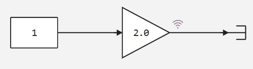
scalar_signal = 1 # Example of a scalar signal # Conclusion 1 -
Vector signal is an ordered set of data of the same type, organized as a vector, which has a direction and can contain several elements.
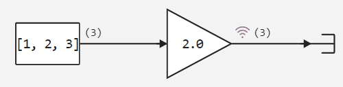
vector_signal = [1, 2, 3] # Example of a vector signal # Conclusion 3-element Vector{Int64}: 1 2 3 -
Matrix signal is a two—dimensional data array consisting of rows and columns, and can contain various types of data. The matrix can be used to represent multiple signals simultaneously.
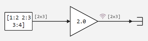
matrix_signal = [1:2 2:3 3:4]

# Conclusion
2×3 Matrix{Int64}:
 1  2  3
 2  3  4
-
-
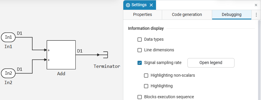
Signal sampling rate — displays the sampling rate of the model blocks. A small sampling step can lead to an increase in the amount of data, which can slow down the execution of the simulation. Taking too large a step can lead to loss of accuracy in calculating the model. Choose the best option based on your model and goals.
Example of displaying the sampling frequency of a signal
-
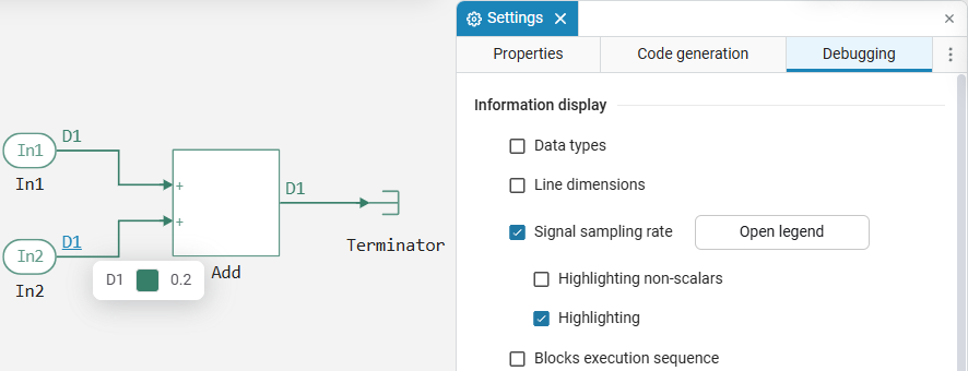
Highlighting — sub-item options Signal sampling rate allows you to color select one of the following options: signals with the current sampling rate, the signal source, or do not select anything (selected by default). Discrete signals can be displayed in different colors depending on the sampling frequency of the signal.
Example of color highlighting
-
-
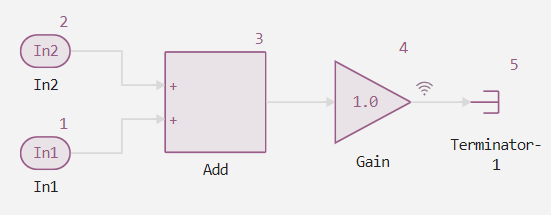
Blocks execution sequence — allows you to find out the order of execution of blocks in the model. The sequence of model execution will be displayed in numbers, where 1 is the first executable block in the model. This option helps to control the sequence of block execution in order to avoid unwanted dependencies and improves the readability of the model.
Example of the execution order
-
-
Record physical variables — allows you to record data from library blocks Physical Modeling. There are three recording settings available:
-
None— disables recording of physical variables. It is used by default if for the parameter Record physical variables the flag is not set. -
Selected blocks— records data only from selected blocks. To enable data recording from the blocks, right-click on the selected block and select in the context menu Log Physical Signals: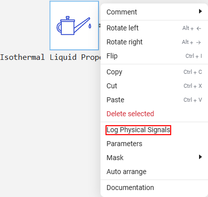
-
All— records data from all library blocks Physical Modeling in the model. In this case, you do not need to record each block individually.The recorded variables are displayed in the window Signal visualization
 and in the app Data Inspector.
-
-
Save simulation results to workspace — allows you to save the simulation results of the model to the workspace (variable window
 ). Read more about saving simulation results in the article Software processing of simulation results in Engee.
 -
Results of physical variables initialization — displays the values of physical variables in the Physical variables window
 .
. -
Enable stepping back — allows you to execute the model one time step at a time. Enabling the setting adds additional buttons to the upper simulation menu Engee:

In this mode, you can configure the parameters:
-
Maximum number of saved back steps — The parameter determines how many simulation steps will be stored in memory. It is useful for understanding how the model reached its current state and for debugging, as it allows you to compare changes at each step.
-
Interval between stored back steps — the parameter sets after how many time steps the state of the model will be saved.
-
Move back/forward by — the parameter determines the number of steps the model will take.:
-
Step forward
 — The simulation continues for the specified number of steps. For example, if the value of the "Step forward/backward by" parameter is
 2then the simulation will advance two steps. -
Step back
 — the simulation returns for the specified number of steps. Engee restores the operating point of the model state, from which the selected number of steps returns.
-
-
-
Showing current signal value — Allows you to mark signals to display the instantaneous value during simulation or step-by-step execution.
-
Animation speed — controls the speed of operation state machine (supported inside the block ChartIt has four modes: off (default), slow, medium and fast.
-
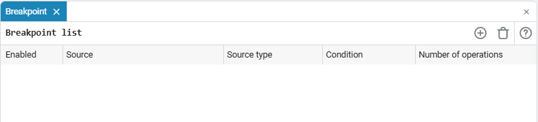
Breakpoint — opens the editor to create points where the execution of the model will be suspended (for more information, see Breakpoints in modeling).