Getting started with solvers in Engee
What is a solver and what is it used for?
Solvers are tools for calculating the dynamic behavior of Engee models. The choice of the solver and its settings significantly affect the accuracy of the final solution and the speed of obtaining it. An unsuccessful option may even lead to an incorrect decision. There is no universal solver for all tasks, so it is important to choose it taking into account the goals of modeling and the features of the model.
|
To view the current solver or select another one, open the window Settings
|
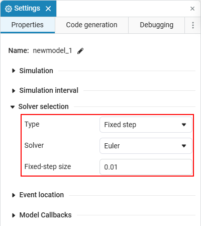
First of all, you need to select the type of solver:
-
Fixed step — the step remains unchanged throughout the computational experiment. They are usually used for real-time calculations or checking the correctness of a numerical solution. In general, they are ineffective due to the fact that the step over the entire modeling interval is limited by the requirements of individual more dynamic sections. Reducing the step to a certain limit increases the accuracy of the solution, but naturally has a negative effect on the calculation speed.;
-
Variable step — automatically adjust the step size during the computational experiment, taking into account changes in the solution and estimates of local integration errors. Such solvers reduce the step in complex areas to maintain accuracy and increase it in simple ones to speed up calculations.
Solvers are also divided into discrete and continuous ones. For models without continuous states (without continuous integrators, transfer functions, etc.), discrete solvers are used, in other cases continuous ones. If one of the continuous solvers is selected for a model without continuous states, then for efficiency it will automatically be replaced with a discrete constant or variable step in accordance with the initial choice. An attempt to calculate a continuous-state model with a discrete solver will result in an error when starting the calculation.
Continuous solvers can be based on various types of numerical methods, among which it is worth highlighting separately:
-
Implicit methods — require solving a system of nonlinear algebraic equations at each step. They are suitable for rigid systems (for more information, see Choosing a solver), as they allow you to use large steps without loss of stability, but each step requires serious computing resources. Examples in Engee: ImplicitEuler, Trapezoid, TRBDF2, RadauIIA5, KenCarp*, Kvaerno*, QNDF*, QBDF*, FBDF;
-
Semi—implicit methods - unlike implicit methods, they require solving a system of linear algebraic equations at each step. As well as implicit ones, they are well suited for rigid systems of equations. In general, they strongly depend on the accuracy of the Jacobi matrix calculation. Examples in Engee: Rosenbrock*, Rodas*;
-
Multistep methods — Use data from several previous steps to calculate the next one. They can be particularly effective for large tasks, but in the presence of multiple events, their speed decreases due to constant reinitialization, so they are not recommended for models with discontinuous components. Examples in Engee: VCABM*, AB*, ABM*, QNDF*, QBDF*, FBDF.
-
— a family of methods, for example, Kvaerno* means Kvaerno3, Kvaerno4, Kvaerno5, etc.
-
Choosing a solver
When calculating a model, it is impossible to achieve high accuracy and speed at the same time. It is necessary to find a balance between these indicators by choosing a suitable solver. To do this, you will need to have a good understanding of the characteristics of the system that it will solve, namely:
-
System rigidity — a rigid model is called a model in which fast and slow processes occur simultaneously, such as in chemical reactions or electromechanical systems. For such models, explicit methods require very small steps due to their small stability range, so it is better to use implicit or semi-implicit methods, the step of which will be limited only by accuracy requirements. A system is considered rigid if its time constants differ by
6and more orders of magnitude; -
Model size is the number of continuous variables that uniquely identify a particular state of the model. A model is considered large if it has more than
1000state variables. The more of them there are, the slower the calculations go, especially when using implicit and semi-implicit methods. For large models, it is better to use methods with fewer calculations of the right-hand side (derivatives of the system) at each step.; -
Requirements for the accuracy of the solution — determine the proximity of numerical and exact solutions. The requirements for absolute and relative accuracy are distinguished separately.:
-
Absolute tolerance (atol) — if the variable is modulo less than this setpoint, the local error estimate for the variable is considered zero. For example, for models with first-order solution components, the value is usually used but in general , this setting is individual for each specific model .;
-
Relative tolerance (rtol) — defines an acceptable local error relative to the variable value itself. Approximate setpoint values:
-
— low accuracy;
-
— High precision;
-
— very high accuracy.
Higher accuracy requires the use of advanced solvers, which can significantly increase the total calculation time.
-
-
-
The presence of gaps in the solution — some library components, for example Abs or Saturation, are characterized by abrupt abrupt changes in behavior, which leads to gaps in the solution. Multistep methods are generally less effective for such tasks.
The following table can be used as a starting point when choosing a variable-step solver:
| Precision/Rigidity | Non-rigid | Moderate hardness | Tough |
|---|---|---|---|
Low |
BS3 |
ROCK2 |
ImplicitEuler, Trapezoid, Rodas3, Rosenbrock23, TRBDF2 Large dimension: TRBDF2 |
Average |
Tsit5, BS5, DP5 Large dimension: VCABM |
ROCK4 |
Rodas4, Rodas4p, KenCapr4 Large dimension: QNDF, QBDF |
High |
DP8, Vern6, Vern7, Vern8, Vern9 Large dimension: VCABM |
Rodas5, Rodas5p, RadauIIA5, Kvaerno5 |
Rodas5, Rodas5p, RadauIIA5, Kvaerno5 Large dimension: QNDF, QBDF |
Since there is no universal solver for all models, you need to select the solver yourself, focusing on the specifics of the problem, the required accuracy and the allowable calculation time. In this case, you can try not only solvers from one cell (in the table above), but also from neighboring cells to find the most optimal option. A rational solution would be to find a balance between performance and quality, which will allow for correct and effective modeling.