Local solvers for physical networks

In Engee The mechanism of local solvers is used to calculate the behavior of physical networks. The system model identifies physical networks connected by directional components such as amplification links, integrators, etc. Each physical network is calculated by its own independent solver, and interpolators are installed at its inputs and outputs. The directional part of the model is controlled by a global solver, and physical networks are perceived by it as ordinary directional components without an internal state.
Local solvers can significantly increase the speed of model calculation without sacrificing much on the quality of the solution. Physical models often contain components of different physical nature, and different physical phenomena occur in them at different speeds. Using local solvers, it is possible, for example, to consider the electrical part of the model with a small step, and the mechanical part with a large one.
On the other hand, electrical circuits are often described by rigid systems of differential equations, while mechanical models are described by non—rigid ones. This makes it possible to use complex methods for electrical circuits, and simpler ones for mechanical circuits. Also, large rigid models can be divided into several parts, each of which will be considered the same implicit or semi-implicit solver.
The time complexity of the decomposition of an NxN Jacobi matrix is . For simplicity, let it be exactly operations. When splitting a large model into two parts, the total number of operations for its calculation is
,
where — overhead costs for interpolators and synchronization of solvers. These costs usually make up a negligible fraction of the total calculation time for at least a slightly complex model. Splitting the initial model into two parts calculated by local solvers, at best, gives a fourfold acceleration of the calculation. In practice, the acceleration turns out to be less due to various factors, but local solvers often allow you to significantly speed up the calculation.
Engee Supports two types of synchronization of local and global solvers: discrete and continuous.
The first type is especially relevant for real-time calculations, for example, on a complex semi-natural RITM simulation. A physical network is represented as a discrete atomic component without a state, for which the sampling period is specified. Two numerical methods are available: the implicit Euler method (ImplicitEuler) and the trapezoid method (Trapezoid). For their operation, it is not necessary to interpolate the input signals, and the output signals are discrete by definition.
In addition to the numerical method, a fast version is chosen (Fast) or reliable (Robust). If a convergence error occurs, you can switch to a reliable version of the algorithm (Robust) or reduce the sampling step. Sometimes it is useful to reduce the sampling step to a multiple of the original value, for example, not with 0.1 before 0.01, and before 0.03 to bypass the problem area.
The simplifications used in the discrete synchronization mode may lead to the model being calculated faster, but the accuracy of the calculation may be insufficient. Then you can reduce the sampling period in the corresponding solver settings window or switch to continuous synchronization.
When continuous synchronization is enabled, the global solver begins to perceive the physical network as a continuous component with no internal state. Its inputs use an interpolation suitable for the selected solver, and its output is a continuous function. It is necessary to set the synchronization interval with which the local and global solvers will exchange information. The local solver can perform as many intermediate steps to the next synchronization point as it needs. This approach improves the accuracy of the calculation, but requires high computational costs.
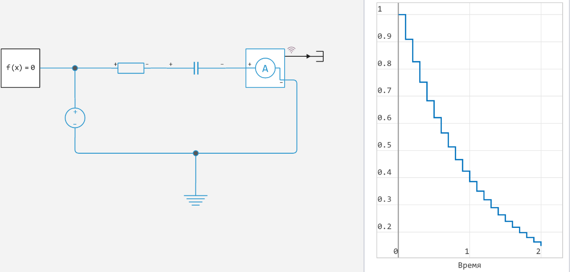
The question arises of breaking algebraic loops — connections of physical networks through directed components without internal states. In this case, an error occurs.:
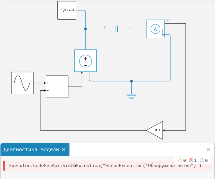
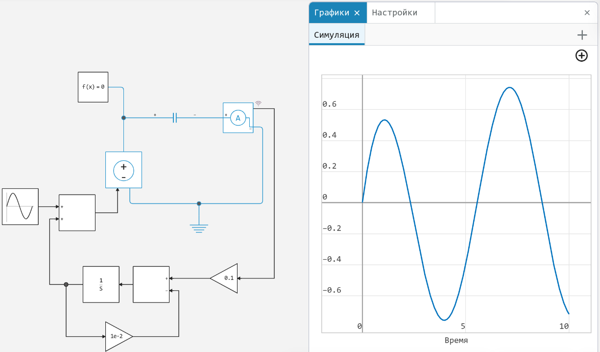
To eliminate it, you can use Unit Delay with a short sampling period:

or an aperiodic link with a suitable time constant:
List of local solvers Engee It is limited to the most useful for calculating physical models and is a subset of global solvers. It is useful to smooth the signals entering the physical network using continuous filters or special functions such as hyperbolic tangent to approximate discontinuous functions.
When selecting continuous synchronization, three types of solvers are available.: Fixed-step, Variable-step and Inherit global. The first two are for fixed and variable steps, and the third inherits the settings of the global solver. This does not mean that the model will be solved by a single global solver. The local solver will receive the same settings as the global one. The latter mode is rarely used in practice, so it is recommended to start with the default settings: continuous synchronization, variable step solver, Rodas4.