Debugging models in Engee
Debugging plays a key role in model development, allowing us to check whether the operation of individual parts of the model and its behavior meet our expectations. This process helps to identify and eliminate errors, verify that the data is transmitted correctly and the dimensions match the intended ones. If an incorrect result occurs at the output of the model, debugging allows you to understand where and how the system behavior deviated from the expected.
The article discusses the main approaches to debugging models using the Engee tools.
Initial debugging of models
At the initial stage of model development, it is important to make sure that its components and connections (signal lines) are working correctly. Initial debugging allows you to identify basic errors, such as incorrect block parameters, incorrect input data, or incorrect execution logic.
Signal graphs
The easiest way to check — mark signals for recording  and observe on the charts where the model starts behaving incorrectly (for more information, see the article Signal visualization).
Disabling and skipping blocks
In the process of debugging models, it often becomes necessary to temporarily exclude some blocks from execution, which is analogous to commenting code in text programming languages.
To disable/skip a block, right-click on it and select the appropriate option in the context menu.:
-
Disable the block — the block is completely excluded from the model, as if it did not exist. Its inputs and outputs are torn apart, and it does not participate in the simulation process in any way. This allows you to check how the model will work without this block. Therefore, if the unit is disabled, then the signal is not transmitted through it, and the components connected to its outputs do not receive data.
-
Skip the block — the block remains in the model, but its functionality is ignored. The inputs of the unit are directly connected to its outputs, and the data passes through unchanged. This is equivalent to connecting all the inputs of the block to the corresponding outputs.
The pass is not available for some blocks.
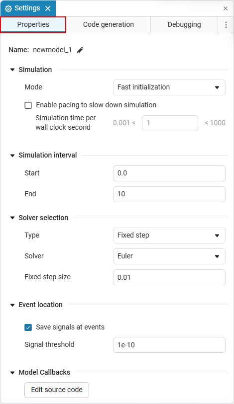
The "Properties" tab of the settings window
Selecting the simulation mode
Parameter Mode allows you to configure the simulation execution depending on debugging tasks and performance. For debugging, the mode is especially useful, which minimizes startup time and simplifies working with the model. There are two modes available in total:
-
Fast initialization — the model starts as quickly as possible due to simplified typing and disabling optimizations. This mode is convenient for debugging, as it allows you to quickly check changes in the model without waiting a long time for startup. It is especially useful for frequent changes in the structure or parameters of the model.
-
Fast simulation — High performance and reduced computing time are given priority. Although this mode is less flexible for debugging, it can be useful in the final stages of verification, when it is necessary to ensure the correctness and stability of calculations.
Therefore, it is recommended to use the mode at the initial stages. Fast initialization to quickly find and fix errors, and on the final — Fast simulation to check the performance of the model.
Simulation speed control
Parameter Enable pacing to slow down simulation allows you to set the ratio of simulation time to real time, specifying how many seconds of simulation should pass in one real second.
This setting is useful for debugging, as slowing down the simulation helps to better analyze the behavior of the model in real time. This allows you to:
Therefore, slowing down the simulation creates a controlled work environment in which you can interact with the model, analyze the behavior of signals, and fix problems in the early stages of debugging.
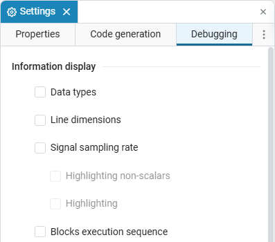
Tab "Debugging" settings windows
Displaying information
When debugging models, it is important to be able to visually track key characteristics in order to understand how data is transmitted and processed in blocks. Various types of information can be displayed in Engee:
-
Data types — displays the data types of the signal lines between the model blocks. If an incorrect data type is present in the model, then when selecting the function Data types It will appear automatically diagnostic window indicating the error.
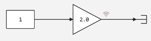
Example of displaying data types
-
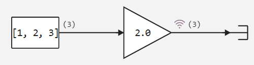
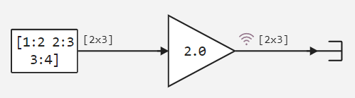
Line dimensions — displays the dimensions of the signal lines between the blocks of the model (read more in Working with signals of different dimensions). Model signals can be scalar, vector, and matrix.
Display examples with different signals
-
Scalar signal is a single data value that has no direction and is the simplest type of signal.:
-
Vector signal is an ordered set of data of the same type, organized as a vector, which has a direction and can contain several elements.
-
Matrix signal is a two—dimensional data array consisting of rows and columns, and can contain various types of data. The matrix can be used to represent multiple signals simultaneously.
-
-
Signal sampling rate — displays the sampling rate of the model blocks. A small sampling step can lead to an increase in the amount of data, which can slow down the execution of the simulation. Taking too large a step can lead to loss of accuracy in calculating the model. To control the sampling frequency of the signal, it is convenient to use the block Rate Transition.
Sample rate example
Here for the block DSP Sine Wave The amplitude is 1, the frequency is 2 Hz, and the sampling step is 0.001 for the first channel (D1, the DSP Sine Wave block) and 0.01 for the second (D2, the DSP Sine Wave-1 block). In the Rate Transition block, the sampling step is set: 0.005 for D1 and 0.02 for D2. This will allow you to see on the graph: the D1 signal is smoothed and accurate, the D2 signal is stepwise, with less detail.
-
Highlighting — sub-item options Signal sampling rate allows you to color select one of the following options: signals with the current sampling rate, the signal source, or do not select anything (selected by default). Discrete signals can be displayed in different colors depending on the sampling frequency of the signal (as in the example above).
-
-
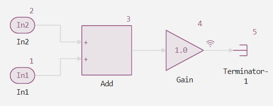
Blocks execution sequence — allows you to find out the order of execution of blocks in the model. The sequence of model execution will be displayed in numbers, where 1 is the first executable block in the model. This option helps to control the sequence of block execution in order to avoid unwanted dependencies and improves the readability of the model.
Example of the execution order
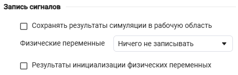
Recording of signals
Recording the signals allows you to capture the simulation results and analyze them for subsequent diagnosis and debugging. There are two ways to record signals in Engee:
-
Save simulation results to workspace — allows you to save the simulation results of the model to the workspace (variable window
 ) as a variable
 simout. This allows you to access the data after the simulation is completed and use it for analysis, visualization, or post-processing. Read more about saving simulation results in the article Software processing of simulation results in Engee.-
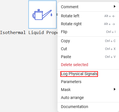
Physical Variables — allows you to record data from selected blocks. Only blocks from the library are suitable for recording Physical Modeling. Right-click on the block you want to record the signal from and select the option Log Physical Signals in the context menu:
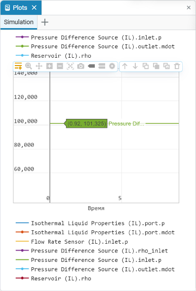
The recorded variables are displayed in the module Plots
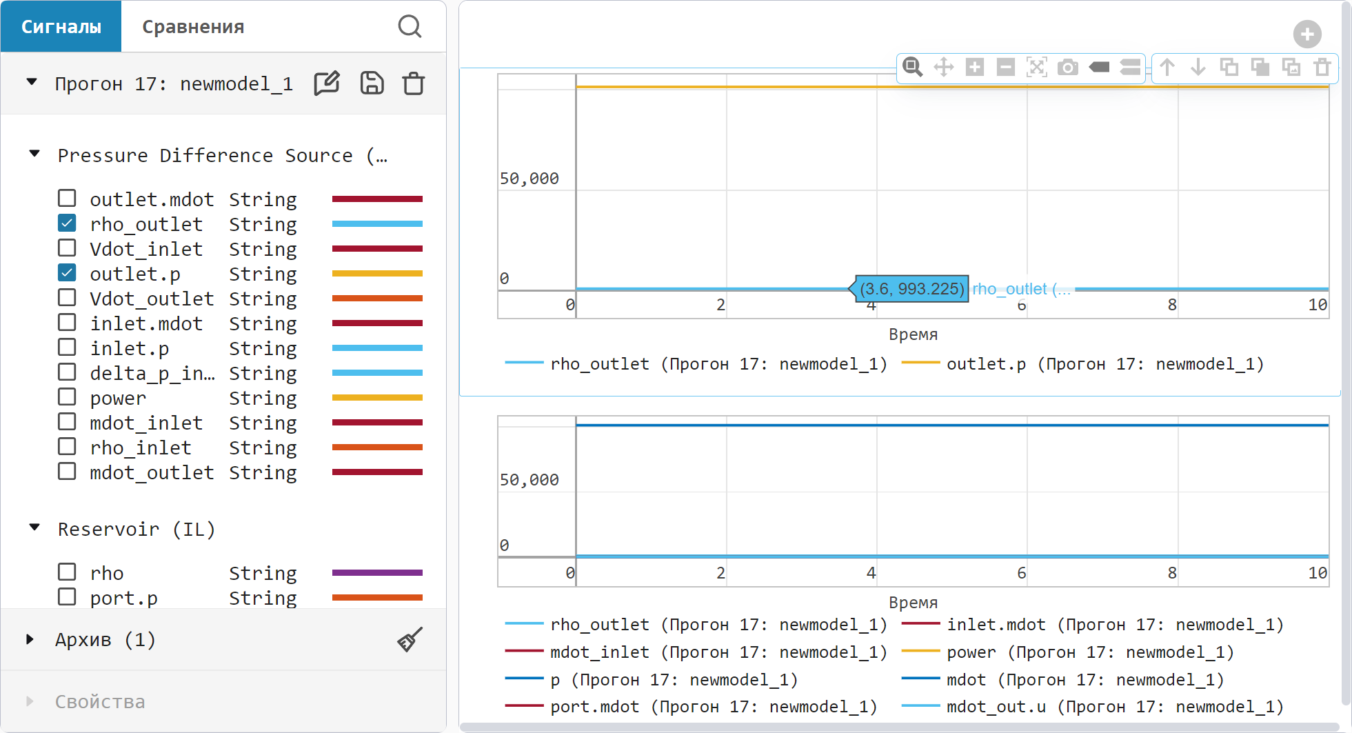
 and in the app Data Inspector.
Examples of recorded signals
Recorded variables in the module Plots:
Recorded variables in the application Data inspector:
-
-
Results of physical variables initialization — displays the values of physical variables in the Physical variables window
 .
.
Real-time debugging
The Engee environment allows you to monitor the execution of the model in real time. This approach combines several tools that help you monitor the status of signals, blocks, and their dynamic processes step by step.:
-
Enable stepping back — allows you to execute the model one time step at a time. Enabling the setting adds additional buttons to the upper simulation menu Engee:

In this mode, you can configure the parameters:
-
Maximum number of saved back steps — The parameter determines how many simulation steps will be stored in memory. It is useful for understanding how the model reached its current state and for debugging, as it allows you to compare changes at each step.
-
Interval between stored back steps — the parameter sets after how many time steps the state of the model will be saved.
-
Move back/forward by — the parameter determines the number of steps the model will take.:
-
Step forward
 — The simulation continues for the specified number of steps. For example, if the value of the "Step forward/backward by" parameter is
 2then the simulation will advance two steps. -
Step back
 — the simulation returns for the specified number of steps. Engee restores the operating point of the model state, from which the selected number of steps returns.
-
-
-
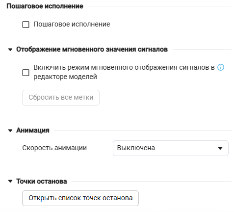
Showing current signal value — Allows you to mark signals to display the instantaneous value during simulation or step-by-step execution. This method is clear and convenient for visual analysis of data transmission between blocks.
-
Animation speed — controls the speed of operation state machine (supported inside the block *Chart*It has four modes: off (default), slow, medium and fast.
Breakpoint
One of the important tools for debugging models is Breakpoint. They allow you to pause the execution of the model at the right moment of the simulation in order to study the state of the system, find errors, or check the operation of individual blocks and settings.
To open the point editor, go to the settings window ![]() and in the tab Debugging choose Open the breakpoint list:
and in the tab Debugging choose Open the breakpoint list:
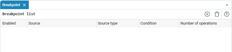
This opens the editor for working with breakpoints.:
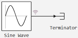
Let’s look at an example where using breakpoints, the simulation stops at a specific stage. To do this, assemble the model from blocks Sine Wave and Terminator, turn on the signal recording:
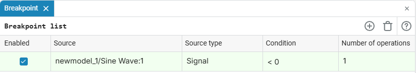
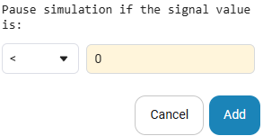
Click the signal line with the left mouse button and click in the breakpoint editor  . In the window that opens, select less than zero as shown in the picture:
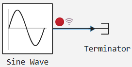
The created breakpoint will have a distinctive red mark on the signal line.:
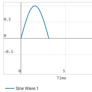
Run the simulation. The simulation will pause on the third second, and the graph of the model will look like this:
The triggered breakpoint will be marked in green in the editor, and the number of triggers will be shown in the column Number of operations: