Signal processing by frames and counts
used terms
|
Sample-based processing
Sample processing — Signals are processed one data element per unit of time. Such processing is characterized by updating the data at each time step, which corresponds to the sampling period. The time step is equal to the period of the step (Sample period), denoted as . The sampling rate is defined as the inverse of the sampling period, i.e. — this means that the data is updated and processed at each step. .
Sample-based processing is better suited for real-time systems that require an immediate response to each new data measurement. Examples of such systems:
-
Audio processing
-
Real-time monitoring
Frame-by-frame processing (Frame-based processing)
Frame—by-frame processing - Signals are processed in frames, where each frame contains several data elements. Frame-by-frame processing updates the data at each time step equal to the frame period. The frame period is defined as the product of the number of elements in the frame ( ) for the sampling period, that is . Accordingly, the frame rate is equal to the sampling rate divided by the number of elements in the frame.: — this allows you to process large amounts of data in a single time step.
Frame-by-frame processing is effective for processing large amounts of data. Usage examples:
-
The Fourier transform
-
Digital filtering
-
Image and video processing
Comparison of treatments by counts and by frames
For clarity, pay attention to the figure, which shows an example of signal processing by samples and frames.:

Comparison table |
|
|---|---|
Processing by counts |
Frame-by-frame processing |
|
|
Thus, it is recommended to start development with frame-by-frame processing, as it is convenient for rapid prototyping and demonstration of the system. Due to its simplicity and speed of development, frame-by-frame processing makes it easy to test and configure algorithms without worrying about the complexities of working with memory. After you are convinced of the correctness of the algorithms and models, you can proceed to processing by counts. This processing, although more complex to implement, provides the high accuracy and optimization needed to work with physical systems that require detailed signal processing and memory interaction. This approach allows you to maximize the benefits of both methods at different stages of development.
Examples
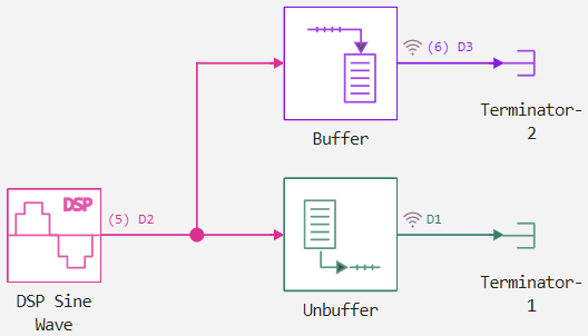
Expand the model from the blocks:
-
DSP Sine Wave — provides a discrete sine wave.
-
Terminator — the block that closes the output port.
-
Buffer — forcibly saves a set number of data elements in one frame. Using the block Buffer the signal is forcibly processed frame-by-frame.
-
Unbuffer — Forcibly converts any number of frames into counts. Using the block Unbuffer the signal is forcibly processed by counting.
-
Turn it on signal recording
 at the output of the blocks DSP Sine Wave, Buffer and Unbuffer.
 -
For clarity, in the settings window
 in the tab Debugging turn it on:
-
Line dimensions
-
Signal sampling rate
-
Highlighting
-
Set the following block parameters:
-
At the block DSP Sine Wave
-
Sample time to the value
0.1; -
Samples per frame to the value
5.
-
-
At the block Buffer
-
Output buffer size (per channel) to the value
6.
-
-
Blocks Unbuffer and Terminator they do not have configurable parameters. In the settings window, the simulation interval and solver selection remain by default.
Run a simulation of the model  . The graphs will show the changes in the sinusoidal signal over time. The X axis represents the simulation time interval from
 0 to 10 seconds, and Y shows the value of the sinusoidal signal. Then in the charts window  will be displayed:
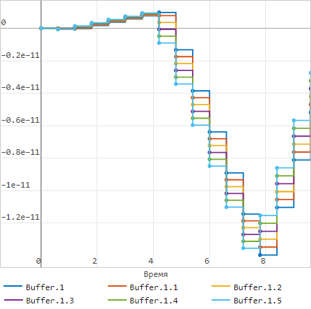
The graph shows the result of the block operation. Buffer, which forcibly saves a set number of data elements in one frame. Each frame contains six data elements represented by colored lines on the graph. These lines represent the state of each element in the frame.
The horizontal stepped line sections show how the values of the data elements remain constant during each frame. The values are updated every 0.6 seconds, which corresponds to the refresh interval of the frame (6 data elements * 0.1 sec/element = 0.6 sec). Block Buffer groups data elements into 6 pieces and displays them as a single frame in which each color corresponds to a specific data element.
In this example, the sample processing is selected, despite the fact that the block Buffer forcibly saves data elements in one frame. This is done to demonstrate the operation of the block and display each data element individually.
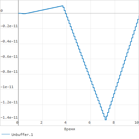
The graph shows the result of the block operation. Unbuffer, which turns any number of frames into counts. Each frame containing 6 data elements is split into separate data elements and transmitted to the block output. Unbuffer one at a time. As a result, the graph shows consecutive data elements of the sinusoidal signal returned to their original discrete form.
The graph is staggered because the values of the data elements change every 0.1 seconds. This corresponds to the time step set for generating a sinusoidal signal. Hence, the block Unbuffer converts the frame-by-frame signal back to a count, which illustrates the reverse process of data buffering.
To switch the graph from countdown to frame-by-frame display, click Signal Menu  in the upper menu of the signal visualization window, select Time domain frame in the upper menu of the signal visualization window, select Time domain frame |
Thus, frame-by-frame and sample processing can have different effects on the representation and processing of signals. Block Buffer Converts samples into frames, grouping data elements and making processing more efficient for tasks that require processing groups of data simultaneously. Block Unbuffer returns frames back to the countdown format.