The relationship of differentials, derivatives and integrals in Engee: from theory to practice

Mathematical analysis is the foundation for many fields of science and engineering. Derivatives and integrals are used in physics, economics, machine learning, and even game AI. Engee, thanks to its performance and user-friendly syntax, is great for numerical computing.

In this article, we will analyze:

How to calculate derivatives and integrals in Engee
Practical application in modeling and optimization
Examples from real projects

1. Derivatives: from mathematics to code

The derivative of the function ( f(x) ) shows the rate of its change. In Engee, it can be calculated analytically (symbolically) or numerically.

*1.1. Numerical differentiation**

Package FiniteDifferences allows you to calculate derivatives using the finite difference method:

Pkg.add("FiniteDifferences")

   Resolving package versions...
  No Changes to `~/.project/Project.toml`
  No Changes to `~/.project/Manifest.toml`

using FiniteDifferences

f(x) = x^2 + sin(x)
df = central_fdm(5, 1)(f, 1.0)  # The derivative at the point x=1
println("f'(1) ≈ ", df)  # ≈ 2.5403 (exact value: 2 + cos(1) ≈ 2.5403)

f'(1) ≈ 2.5403023058683987

Application in real projects:

In physics, the calculation of acceleration (the derivative of velocity).
In economics, marginal costs (the derivative of the cost function).

1.2. Automatic Differentiation (AD)

Engee supports auto-differentiation via ForwardDiff:

using ForwardDiff

f(x) = 3x^3 + 2x^2 + x
df_analytical(x) = ForwardDiff.derivative(f, x)

println("f'(2) = ", df_analytical(2))  # Outputs 45

f'(2) = 45

Where is it used?

Optimization in machine learning (gradient descent).
Numerical solution of differential equations.

2. Integrals: from summation to modeling

The integral is the "area under the curve". In Engee, it can be calculated numerically.

2.1. Numerical integration

Package QuadGK implements the Gauss-Kronrod method:

Pkg.add("QuadGK")

   Resolving package versions...
  No Changes to `~/.project/Project.toml`
  No Changes to `~/.project/Manifest.toml`

using QuadGK

f(x) = exp(-x^2)
integral, err = quadgk(f, 0, 1)
println("∫e^{-x²}dx ≈ ", integral)
println("Error estimate: ", err)

∫e^{-x²}dx ≈ 0.746824132812427
Error estimate: 7.887024366937112e-13

Usage examples:

Finance: calculation of discounted cash flows.
Physics: Calculation of force work.

*2.2. Integration of odes (differential equations)**

Package DifferentialEquations.jl solves complex dynamic systems:

Pkg.add("DifferentialEquations")

using DifferentialEquations

# Predator-prey model (Lotka-Volterra)
function lotka_volterra!(du, u, p, t)
    x, y = u
    α, β, δ, γ = p
    du[1] = α*x - β*x*y  # dx/dt
    du[2] = δ*x*y - γ*y  # dy/dt
end

u0 = [1.0, 1.0]          # Initial conditions: [prey, predators]
tspan = (0.0, 10.0)       # Time interval
p = [1.5, 1.0, 1.0, 3.0] # Model Parameters

prob = ODEProblem(lotka_volterra!, u0, tspan, p)
sol = solve(prob, Tsit5())

using Plots
plot(sol, xlabel="Time", ylabel="Population", label=["Victims" "Predators"])

Where is it applied?

Biology: Population modeling.
Engineering: calculation of system dynamics.

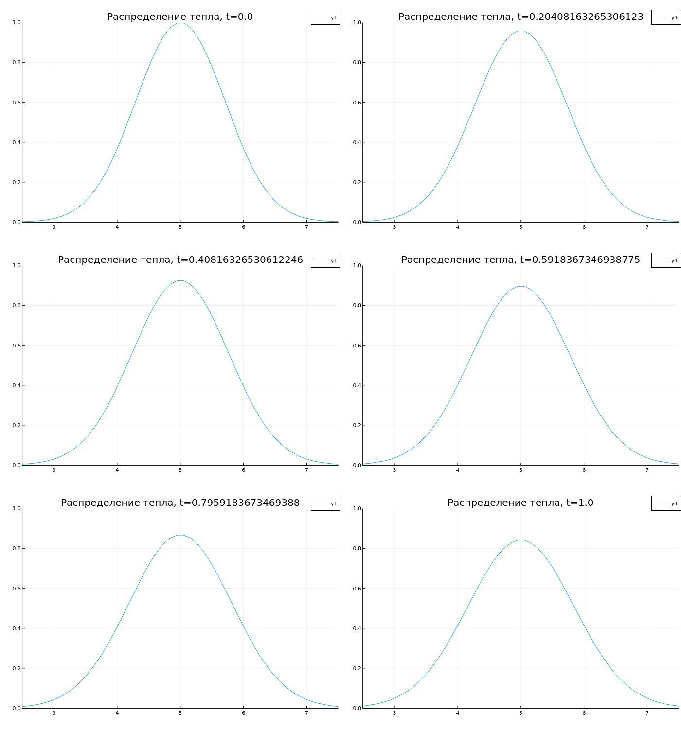
3. The relation of derivatives and integrals: the equation of thermal conductivity

Consider the equation of thermal conductivity:
∂T/∂t = a·∇2T+ qᵥ/(c·p)

where:
a = λ/(cρ) is the thermal conductivity coefficient [m2/s]
∇2 is the Laplace operator (∂2/∂x2 + ∂2/∂y2 + ∂2/∂z2)

Numerical solution in Engee:

using DifferentialEquations

# Setting the grid
L = 10.0
nx = 100
dx = L / nx
x = range(0, L, length=nx)

# Initial condition (hot middle)
u0 = exp.(-(x .- L/2).^2)

# The function for the right side of the equation
function heat_equation!(du, u, p, t)
    α = p
    for i in 2:nx-1
        du[i] = α * (u[i+1] - 2u[i] + u[i-1]) / dx^2
    end
    du[1] = du[end] = 0  # Boundary conditions
end

# We decide
prob = ODEProblem(heat_equation!, u0, (0.0, 1.0), 0.1)
sol = solve(prob, Tsit5())

# Visualization
anim = @animate for t in range(0, 1, length=50)
    plot(x, sol(t), ylims=(0,1), xlims=(2.5,7.5), title="Heat distribution, t=$t")
end
gif(anim, "heat.gif", fps=10)

[ Info: Saved animation to /user/my_projects/Demo/heat.gif

Application:

Physics: simulation of heat transfer.
Finance: calculation of options (Black-Scholes equation).

Conclusion

Engee provides powerful tools for working with derivatives and integrals:

ForwardDiff — for gradients and optimization.
QuadGK — for numerical integration.
DifferentialEquations.jl — for modeling dynamic systems.

These methods are used in:

Physics (heat transfer, mechanics)
Economics (optimization, forecasting)
Data Science (model learning, diffusion processes)