EngeePhased.NonlinearFMWaveform
A signal generator with nonlinear frequency modulation.
| Library |
|
| Block |
Description
System object EngeePhased.NonlinearFMWaveform creates a signal with nonlinear frequency modulation (NFMW). LFM signals allow for low-frequency side lobes due to the nonlinear dependence of time and frequency. Four different signals are supported depending on the property FrequencyModulation:
-
"Polynomial"— generates a signal with an instantaneous frequency that corresponds to a polynomial function. -
"Hyperbolic"— generates a hyperbolic FM signal. -
"Hybrid Linear-Tangent"— generates a hybrid LFM signal combining linear FM and tangential FM. -
"Stepped Price"— generates a signal with a stepwise nonlinear FM Price.
To generate a signal, follow these steps:
-
Create an object EngeePhased.NonlinearFMWaveform and set its properties.
-
Call the object with arguments as if it were a function.
To learn more about how to work with system objects, see Engee System Objects.
Syntax
Creation
-
waveform = EngeePhased.NonlinearFMWaveform()— creates a system object of a signal generator with a nonlinear FMwaveformwith default properties. By default, the signal has a polynomial FM. -
waveform = EngeePhased.NonlinearFMWaveform(Name=Value)— creates a system object of a signal generator with a nonlinear FMwaveformwith the specified properties as a pairName=Value, whereName— the name of the property, andValue— the appropriate value. You can specify multiple pairs «name-value» the order of the pairs does not matter. Unspecified properties retain their default values.
Using
-
Y = waveform()— returns a signal with a nonlinear FM in the form of a column vector Y. The Y argument can contain either a certain number of pulses or a certain number of samples. -
Y = waveform(prfidx)— uses the prfidx index to select the pulse repetition rate (PRF) from a predefined vector of values set by the PRF property. This syntax applies if the PRFOutputPort property is set totrue. Use this syntax in cases where the transmitted pulse needs to be dynamically selected. In such situations, the PRF property includes a list of predefined PRF options. During the simulation, using prfidx, one of the PRF options is selected as the PRF for the next transmission. Note that the transmission always completes the current pulse before starting the next one. Therefore, if you set the property to OutputFormat value"Samples", and then specify the property [Property:numSamples] shorter than the pulse, it is possible that at this modeling step, if the entire output signal is needed to complete the previously transmitted pulse, the specified prfidx will be ignored. -
Y = waveform(freqoffset)— uses freqoffset to generate a frequency offset signal. Use this syntax in cases where it is necessary to dynamically update the frequency of transmitted pulses. This syntax applies if for the property FrequencyOffsetSource value set"Input port". -
Y,PRF = waveform(_)— also returns the current pulse repetition rate PRF. To use this syntax, set the PRFOutputPort property totrue, and for the property OutputFormat value"Pulses". -
Y,coeff = waveform(_)— also returns the coefficients of the matched coeff filter for the current pulse. To use this syntax, set the [Property:CoordicientsOutputPort] valuetrue.
You can combine optional input and output arguments if properties are specified that include them. Optional inputs and outputs should be listed in the same order as the properties that include them. For example, Y,PRF,coeff = waveform(prfidx,freqoffset).
Arguments
Input arguments
prfidx — pulse repetition rate index
+
a positive integer
Details
Pulse Repetition rate index (PRF), set as a positive integer. The index identifies entries in the PRF property. Use this argument in cases where the transmission pulse must be selected dynamically. In such situations, the PRF property contains a list of predefined PRF selection options. During the simulation, based on the input data prfidx, one of the PRFs is selected as the PRF for the next transmission.
Dependencies
To use this argument, set the PRFOutputPort property to true.
freqoffset — frequency offset, Hz
+
scalar
Details
The frequency offset specified as a scalar. The offset allows you to generate a signal with a frequency offset. Use this argument in cases where it is necessary to dynamically update the frequency of the transmitted pulse.
Dependencies
To use this argument, set the property to FrequencyOffsetSource value "Input port".
| Типы данных |
|
Output arguments
Y — pulse signal
+
column vector
Details
The output signal returned as a column vector.
| Типы данных |
|
PRF —
pulse repetition
rate
scalar
Details
Pulse repetition rate in Hz, returned as a scalar. PRF contains the current pulse repetition rate used by the system.
Dependencies
To use this argument, set the PRFOutputPort property to true, and for the property OutputFormat value "Pulses".
| Типы данных |
|
| Support for complex numbers |
yes |
coeff — coefficients of the matched filter
+
vector | the matrix
Details
Coefficients of the matched filter returned as a complex vector of size or a complex matrix of size .
Dependencies
To use this argument, set the property to [Property:CoordicientsOutputPort] value true.
| Типы данных |
|
| Support for complex numbers |
yes |
Features
#
NumSteps —
number of frequency steps
Real number
Details
The number of frequency steps for stepwise nonlinear frequency modulation of the Price, specified as a positive integer.
Default value — 50.
Dependencies
To use this property, set the FrequencyModulation value "Stepped Price".
#
LinearTangentBalance —
the balance coefficient between linear frequency modulation and frequency modulation according to the tangential law
Real number
Details
The dimensionless balance coefficient between linear frequency modulation and tangential frequency modulation, defined as a scalar.
Default value — 0.5.
Dependencies
To use this property, set the FrequencyModulation value "Hybrid Linear-Tangent".
#
SweepInterval —
frequency deviation interval
String
Details
The frequency deviation interval, set as "Positive" (by default) or "Symmetric":
-
"Positive"— the frequency of the signal will vary from0beforeB, whereB— the width of the deviation band in the SweepBandwidth. -
"Symmetric"— the frequency of the signal will vary from−B/2beforeB/2.
#
BandwidthFactors —
bandwidth coefficients
Scalar / vector / matrix of real numbers
Details
Bandwidth coefficients for stepwise nonlinear frequency modulation of the Price, specified as a two-element positive vector of the form [BL BC]. Meaning BL determines the bandwidth of the linear component of the signal, and BC — the bandwidth of the nonlinear component. The total frequency deviation band is , where — the value of the property NumSteps. As you increase the bandwidth of the linear component is approximately equal to BL while the bandwidth of the nonlinear component increases with increasing .
Default value — [1e4 2e4].
Dependencies
To use this property, set the FrequencyModulation value "Stepped Price".
#
OutputFormat —
output signal format
String
Details
The format of the output signal in the form "Pulses" (by default) or "Samples":
-
If you set the value for this property
"Pulses", then the output of the block consists of several pulses. The number of pulses is the value of the property NumPulses. -
If you set the value for this property
"Samples", then the output of the block consists of several samples. The number of samples is the value of the [Property:numSamples] property.
#
NumSamples —
number of samples of the output signal
Real number
Details
The number of samples of the output signal, set as a positive integer.
Default value — 100.
Dependencies
To use this property, set the OutputFormat value "Samples".
#
PolynomialCoefficients —
coefficients of a polynomial function
Scalar / vector / matrix of real numbers
Details
Coefficients of the polynomial frequency function, given as a real vector of length . The vector represents the coefficients of the polynomial - th degree. The first element in Polynomials is the coefficient of the highest degree term . The last element is the coefficient of the zero—degree term.
Default value — [1 0 0].
Dependencies
To use this property, set the FrequencyModulation value "Polynomial".
#
FrequencyOffsetSource —
The source of the frequency offset setting
String
Details
The source of the frequency offset setting, set as "Property" (by default) or "Input port":
-
If the value is set to
"Property", then the offset is determined by the value of the FrequencyOffset. -
If the value is set to
"Input port", the offset is determined by the value of the FreqOffset argument.
#
DutyCycle —
fill factor
Real number
Details
A dimensionless fill factor specified as a scalar in the range [0, 1]. The pulse width is the value of the DutyCycle property divided by the value of the PRF property. This value is dimensionless.
Default value — 0.5.
Dependencies
To use this property, set the DurationSpecification property to "Duty cycle".
#
SweepDirection —
frequency deviation direction of the frequency modulation range
String
Details
The direction of frequency deviation of a signal with nonlinear frequency modulation:
-
"Up"(by default) — increase the frequency. -
"Down"— frequency reduction.
#
Envelope —
the envelope of a frequency-modulated signal
String
Details
The envelope of a frequency-modulated signal, defined as "Rectangular" (by default), "Gaussian", "Hamming", "Chebyshev", "Hann", "Kaiser" or "Taylor".
#
NumPulses —
number of output signal pulses
Real number
Details
The number of pulses of the output signal, set as a positive integer.
Default value — 1.
Dependencies
To use this property, set the OutputFormat value "Pulses".
#
PRF —
pulse repetition rate
Real number
Details
Pulse repetition rate (PRF), set as a scalar or string vector. The units of measurement are Hz. The pulse repetition period (PRI) is the inverse of the pulse repetition rate (PRF). The PRF value must satisfy the following constraints:
-
The product of PRF and PulseWidth must be less than or equal to one. This condition requires that the pulse width be less than one PRI. For a phase-coded signal, the pulse duration is equal to the product of the duration of one chip and the number of chips.
-
Relation SampleRate k PRF must be an integer. This condition requires that the number of samples in one PRI be an integer.
The PRF value can be set using only the PRF property values or the property values combined with the prfidx input argument.
-
If PRFOutputPort has a value
false, PRF is set only using the PRF properties. You can:-
Implement a constant PRF by specifying the PRF property as a positive real scalar value.
-
Implement a discrete PRF by specifying the PRF property as a vector string with positive real elements. Each object call uses consecutive elements of this vector as a PRF. As soon as the object reaches the last element of the vector, it cyclically continues the process with the first element of the vector.
-
-
When PRFOutputPort has a value
trueyou can set the value of PRF using the PRF property in combination with the input argument prfidx. You implement a selectable PRF by specifying the PRF property as a vector string with positive real elements. When executing an object, the PRF is selected using the index specified in the input argument prfidx to index the PRF vector.
In all cases, the number of output samples is fixed if you set the property to OutputFormat value "Samples". When using a variable pulse repetition rate (PRF) and setting for the property OutputFormat values "Pulses" the number of counts may vary.
Default value — 10e3.
#
SweepBandwidth —
frequency deviation
Real number
Details
The bandwidth of a nonlinear frequency-modulated signal, specified as a positive scalar. The units of measurement are Hz.
Default value — 10e4.
#
EnvelopeSidelobeLevel —
the level of the side lobes of the envelope window
Real number
Details
The level of the side lobes of the Kaiser, Chebyshev, or Taylor window used as the envelope of the signal is set as a positive scalar. The units of measurement are dB.
Default value — 30.
Dependencies
To use this property, set the Envelope value "Kaiser", "Chebyshev" or "Taylor".
#
TangentCurvePortion —
section of the tan(x) curve
Real number
Details
Section of the curve between −π/2 and +π/2, used as a tangential term in a hybrid linear-tangential frequency modulation function, defined as a scalar in the range from 0 before +π/2.
Default value — 1.4.
Dependencies
To use this property, set the FrequencyModulation value "Hybrid Linear-Tangent".
#
CoefficientsOutputPort —
enable output of matched filter coefficients
Logical
Details
Enable or disable the output of the coefficients of the matched filter by specifying the value false (by default) or true. Set this property to true to enable the output of matched filter coefficients for the waveform used during the simulation.
#
FrequencyModulation —
a type of nonlinear frequency modulation
String
Details
A type of nonlinear frequency modulation:
-
"Polynomial"(by default) — the frequency of the signal at the output of the block is generated by a polynomial function. The coefficients of the polynomial are set in the property [Property:Polynomials]. The resulting frequency function is normalized so that each pulse occupies the frequency band specified in SweepBandwidth. Property SweepDirection is not used if FrequencyModulation is set to"Polynomial". -
"Hyperbolic"— the unit generates a hyperbolic frequency modulated signal. Use the HyperbolicStartFrequency property to set the initial frequency of the hyperbolic pulse. Property SweepInterval is not used in this case. -
"Hybrid Linear-Tangent"— the unit generates a hybrid waveform combining linear frequency modulation and frequency modulation according to the tangential law [1]. The balance between linear frequency modulation and frequency modulation according to the tangential law is set in the property LinearTangentBalance, and part of the curve , used for the tangential law of modulation, is set in the property TangentCurvePortion. -
"Stepped Price"— the block generates a stepwise version of the nonlinear frequency modulation of the Price [2]. In this case, the property SweepBandwidth is not used, and the frequency deviation is determined by the bandwidth coefficients specified in the BandwidthFactors, and the number of frequency steps in the property NumSteps.
#
PulseWidth —
pulse duration
Real number
Details
The pulse duration, set as a positive scalar. The value must meet the condition PulseWidth < 1/PRF. The units of measurement are seconds.
Default value — 50e−6.
Dependencies
To use this property, set the DurationSpecification property to "Pulse width".
#
SampleRate —
sampling rate
Real number
Details
The sampling frequency of the signal, set as a positive scalar. The ratio of the sampling rate to the pulse repetition rate must be a positive integer, so the number of samples in each pulse must be an integer. The units of measurement are Hz.
Default value — 100e3.
#
HyperbolicStartFrequency —
the initial frequency of the hyperbolic pulse
Real number
Details
The initial frequency of a hyperbolic pulse of a frequency-modulated signal, given as a positive scalar. The units of measurement are Hz.
Default value — 200e3.
#
DurationSpecification —
pulse duration setting method
String
Details
The method of setting the pulse duration in the form "Pulse width" (by default) or "Duty cycle":
-
"Pulse width"— the pulse duration is set using the property PulseWidth. -
"Duty cycle"— the pulse duration is calculated from the values of the properties PRF and DutyCycle. The pulse width is equal to the value of the property DutyCycle divided by the value of the property PRF.
#
PRFOutputPort —
enable PRF output
Logical
Details
If you set the value for this property true. you can pass an index argument to an object to select a predefined value from a vector of property values PRF. If you set the value for this property false (by default), the object will use the PRF property to define the PRF sequence used in the simulation.
#
FrequencyOffset —
frequency offset
Real number
Details
The frequency offset specified as a scalar. The units of measurement are Hz.
Default value — 0.
Dependencies
To use this property, set the FrequencyOffsetSource value "Property".
Examples
Formation of an NLCHM signal with a hyperbolic law
Details
Let’s form an NLCHM signal with a hyperbolic law, pulse duration 50 ms, the initial frequency 10 kHz and the final frequency 500 Hz.
Initialize the parameters.
fs = 20e3 # Частота дискретизации (Гц)
dur_spec = "Pulse width" # Метод формирования длительности импульсов
τи = 50e-3 # длительность импульса (с)

Q = 1 # скважность
prf = round(1/(Q*τи)) # Частота повторения импульсов (Гц)

freq_off_type = "Property" # способ задания параметров "Property" — в параметрах СО
freq_off = 0 # значение начальной частоты спектра (Гц)
out_type = "Pulses" # тип выходного сигнала "Pulses" — по импульсам
num_pulses = 1 # количество импульсов

f1 = 10e3 # начальная частота девиации
f2 = 0.5e3 # конечная частота спектра
Δf = f1 - f2 # ширина спектра НЛЧМ-сигнала
sw_dir = "Down" # направление изменения частоты
type_modulate = "Hyperbolic";
Let’s use EngeePhased.NonlinearFMWaveform to create a probing signal system object nlfm_poly_waveform.
nlfm_poly_waveform = EngeePhased.NonlinearFMWaveform(
    SampleRate = fs, # частота дискретизации
    PulseWidth = τи, # длительность импульса
    SweepBandwidth = Δf, # девиация частоты
    FrequencyModulation = type_modulate, # тип модуляции
    HyperbolicStartFrequency = f1, # начальное значение частоты
    SweepDirection = sw_dir, # направление изменения частоты
    PRF = prf, # частота следования импульсов
    OutputFormat = out_type,
    NumPulses = num_pulses
);
Making a call to the system object EngeePhased.NonlinearFMWaveform using the nlfm_poly_waveform variable:
nlfm_signal = nlfm_poly_waveform();Using the function plot Let’s construct an oscilloscope in the form of an IQ component, a module, and a phase of the signal.
# построение IQ-компонент
t_grid = range(start = 0,step = 1/fs,length = length(nlfm_signal)) * 1e6 # сетка времени, мкс
fig1 = plot(t_grid,real.(nlfm_signal),title = "синфазная составляющая",lab="",ylab="Амплитуда")
fig2 = plot(t_grid,imag.(nlfm_signal),title = "квадратурная составляющая",lab="",xlab = "Время, мкс",ylab="Амплитуда");

plot(fig1,fig2,layout = (2,1))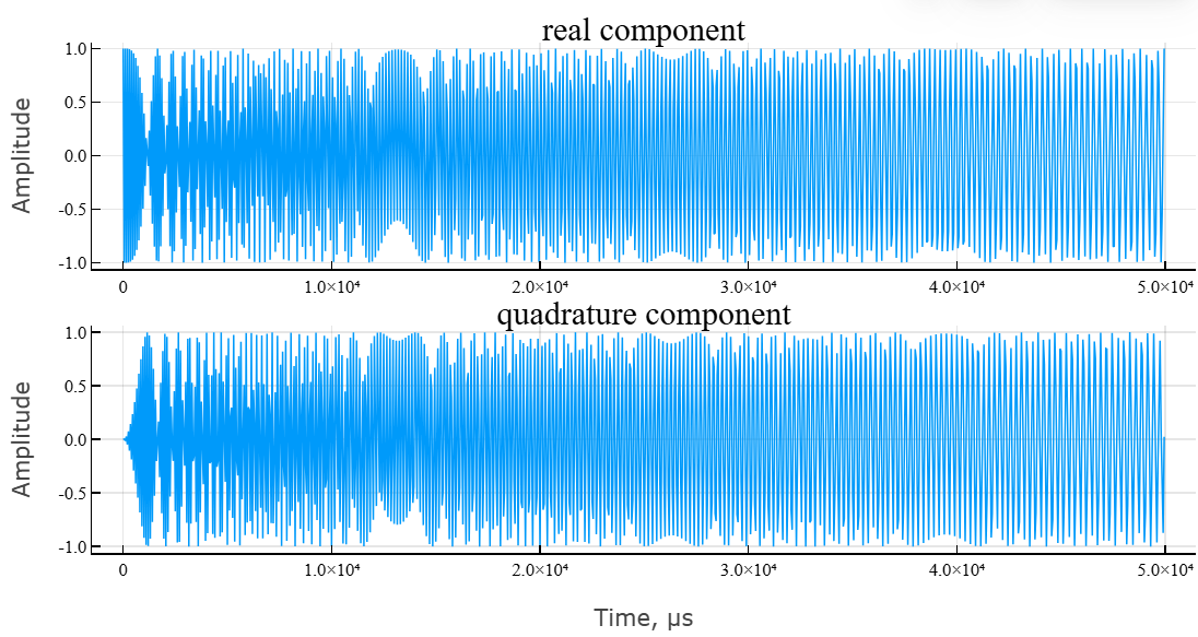
# построение модуля и фазы сигнала
fig3 = plot(t_grid,abs.(nlfm_signal),title = "Модуль комплексного сигнала",lab="",ylab="Амплитуда",ylim = (0,1.2));
fig4 = plot(t_grid,angle.(nlfm_signal)*180/pi,title = "Аргумент комплексного сигнала",lab="",xlab = "Время, мкс",ylab="Фаза, град.");

plot(fig3,fig4,layout = (2,1))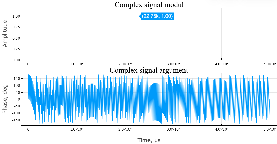
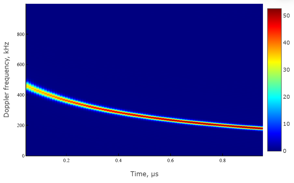
The main characteristic of the signal is the frequency spectrum and the spectrogram. Let’s use the built-in function periodogram.
# расчет спектра сигнала
spec_NLFM,f = EngeePhased.Functions.periodogram(
    nlfm_signal, # исходный сигнал
    ones(size(nlfm_signal)...),
    8192; # длина частоты дискретизации
    out = :data, # тип выхода
    fs = fs, # частота дискретизации
    spectrumtype = "power" # тип спектра
);
Visualize the result using the function plot.
plot(
    f * 1e-3,
    EngeePhased.Functions.mag2db.(spec_NLFM),
    lab="", xlab = "Частота, кГц",
    ylab = "Мощность, дБВт",
    title = "Спектр сигнала"
)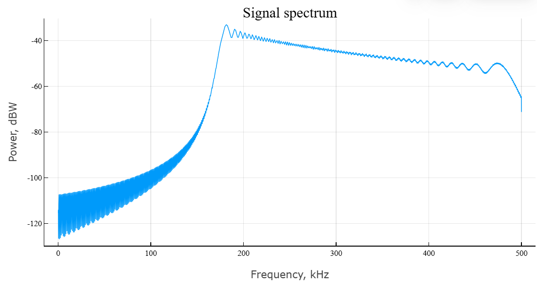
The spectrum is centered around a central frequency , with a stripe . To calculate the spectrogram, we use the built-in function spectrogram.
# расчет спектрограммы
spectgm_nlfm,f1,t1 = EngeeDSP.Functions.spectrogram(
    nlfm_signal;
    nfft = 1024, # длина БПФ
    window = 100,
    noverlap = 90, # перекрытие окна
    spectrumtype = "power",  # тип спектра — по мощности
    freqrange = "twosided", # диапазон спектра — двусторонний
    out = :data, # тип выхода — массив данных
    fs = fs # частота дискретизации
);
We visualize the result of the spectrogram calculation using the function heatmap.
# построение спектрограммы
heatmap(
    t1[:]*1e3,
    f1[:]*1e-3,
    abs.(spectgm_nlfm),color = :jet,
    xlab = "Время, мс",
    ylab = "Частота Доплера, кГц",
)
Algorithms
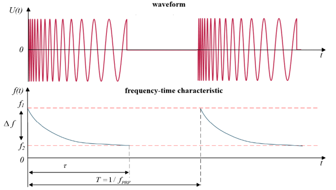
The NLFM radio pulse can be written as
where
-
— pulse duration;
-
— nonlinear phase change law (for example, hyperbolic or symmetric tangential law).
To generate a signal with nonlinear frequency modulation, the following parameters must be set:
-
filter sampling rate ;
-
pulse duration ;
-
pulse repetition rate ;
-
number of pulses ;
-
the initial frequency of the signal ;
-
the final frequency of the signal ;
-
frequency deviation .
The figure shows an NLFM signal with a hyperbolic law. .
Literature
-
Collins, T., and P. Atkins. Nonlinear frequency modulation chirps for active sonar. IEE Proceedings-Radar, Sonar and Navigation 146.6 (1999): 312–316.
-
Levanon, Nadav, and Eli Mozeson. Radar signals. John Wiley & Sons, 2004, pp. 92–93.
-
Doerry, Armin Walter. Generating nonlinear FM chirp waveforms for radar. No. SAND2006-5856. Sandia National Laboratories (SNL), Albuquerque, NM, and Livermore, CA (United States), 2006.
-
Cook, C. E. A class of nonlinear FM pulse compression signals. Proceedings of the IEEE 52.11 (1964): 1369–1371.
-
Yang, J., and T. K. Sarkar. Doppler‐invariant property of hyperbolic frequency modulated waveforms. Microwave and optical technology letters 48.6 (2006): 1174–1179.
-
Melvin, William L., and James Scheer. Principles of modern radar: advanced techniques. SciTech Pub., 2013.
-
Alphonse, Sebastian, and Geoffrey A. Williamson. Evaluation of a class of NLFM radar signals. EURASIP Journal on Advances in Signal Processing 2019.1 (2019): 1–12.