spline
Cubic spline data interpolation.
| Library |
|
Arguments
Input arguments
# x — coordinates of x
+
vector
Details
Coordinates x, set as a vector. Vector x defines the points where the data is set y. Elements x they must be unique.
Cubic spline interpolation requires at least 4 points. If available 2 or 3 Linear or quadratic interpolation is applied to the points, respectively.
| Data types |
|
# y is the value of the function at the specified coordinates x
+
vector | the matrix | array
Details
Function values in coordinates x, specified as a numeric vector, matrix, or array. Arguments x and y they usually have the same length, but y it can also have exactly two more elements than x, to specify the final slopes.
If y — a matrix or an array, then the values in the last dimension, y(:,…,:,j), are taken as values to be compared with x. In this case, the last dimension is y must have the same length as x, or have exactly two more elements.
The final slopes of a cubic spline follow the following rules:
-
If
xandy— the vectors are the same size, then the conditions "not a node" are used. -
If
xoryIf is a scalar, then it expands to the same length as the other one, and the conditions "not a node" are used. -
If
y— a vector containing two elements more values thanx, then the spline uses the first and last values inyas the final slopes of a cubic spline. For example, ify— vector, then: -
Similarly, if
y— the matrix or -a dimensional array with the sizesize(y,N), equal tolength(x)+2Then:
| Data types |
|
Output arguments
# s — interpolated values at query points
+
scalar | vector | the matrix | array
Details
The interpolated values at the query points returned as a scalar, vector, matrix, or array.
# pp is a piecewise polynomial
+
structure
Details
A piecewise polynomial returned as a structure. The structure contains the fields shown in the table.
| Field | Description |
|---|---|
|
|
|
Length vector with strictly increasing elements representing the beginning and the end of each of the intervals |
|
Matrix size on , in which each line |
|
Number of parts |
|
Degree of polynomials |
|
Dimension of the goal |
Since the coefficients of the polynomials in coefs are the local coefficients for each interval, it is necessary to subtract the lower bound of the corresponding node interval in order to use the coefficients in the usual polynomial equation. In other words, for the coefficients on the interval the corresponding polynomial is:
Examples
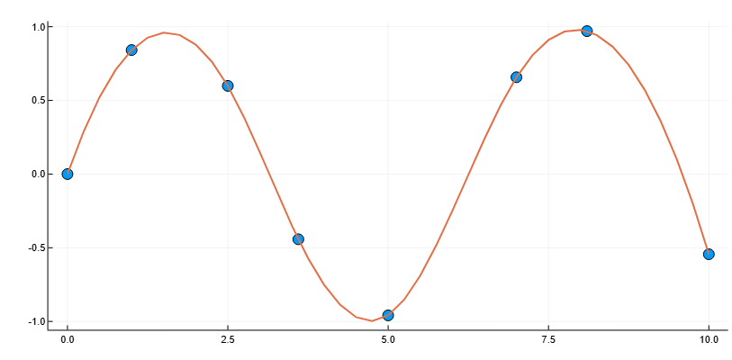
Spline interpolation of sinusoidal data
Details
We use spline to interpolate a sinusoidal curve over unevenly spaced sampling points.
import EngeeDSP.Functions: spline
x = [0, 1, 2.5, 3.6, 5, 7, 8.1, 10]
y = sin.(x)
xx = 0:0.25:10
yy = spline(x, y, xx)

plot(x, y, seriestype=:scatter, markersize=6, legend=false)
plot!(xx, yy, linewidth=2, legend=false)