modalfit
Modal parameters derived from frequency characteristics.
| Library |
|
Syntax
Function call
-
fn,dr,ms,ofrf = modalfit(frf,f,fs,mnum,out=:data)— evaluates the natural frequencies of modesmnumsystems with measured frequency characteristicsfrfdefined at frequenciesf, for the sampling ratefs. Usemodalfrfto build a frequency response matrix based on the measured data. It is assumed that the matrixfrfIt is presented in the format of dynamic flexibility (receptivity).
-
modalfit(_,out=:plot)— plots frequency characteristics.
Arguments
Input arguments
# frf — frequency characteristics
+
vector | the matrix | array
Details
Frequency characteristics specified as a vector, matrix, or array. Argument frf has a size of on on , where — number of frequency intervals, — the number of response signals, and — the number of excitation signals.
Use modalfrf to build a frequency response matrix based on the measured data.
| Типы данных |
|
| Support for complex numbers |
Yes |
# fs is the sampling rate of the measurement data
+
positive scalar
Details
The sampling frequency of the measurement data in Hz, set as a positive scalar.
| Типы данных |
|
# mnum — number of mods
+
a positive integer
Details
The number of modes specified as a positive integer.
| Типы данных |
|
Input arguments «name-value»
Specify optional argument pairs as Name,Value, where Name — the name of the argument, and Value — the appropriate value. Type arguments «name-value» they should be placed after the other arguments, but the order of the pairs does not matter. You can specify multiple pairs «name-value».
Use commas to separate the name and value, and Name enclose it in quotation marks, or use an equal sign to separate the name and value, and Name specify it without quotation marks.
Example: modalfit(frf,f,fs,mnum,"FitMethod","pp","FreqRange",[0 500]) or modalfit(frf,f,fs,mnum, FitMethod="pp",FreqRange=[0 500]) uses a peak extraction method to perform an approximation and limits the frequency range from 0 before 500 Hz.
# Feedthrough — the presence of a gap in the estimated transfer function
+
false (by default) | true
Details
The presence of a gap in the estimated transfer function, set as a Boolean value. This argument is only available if for the argument FitMethod the value is specified "lsrf".
| Типы данных |
|
# FitMethod — approximation method
+
"lsce" (by default) | "lsrf" | "pp"
Details
The approximation method, defined as "lsce", "lsrf" or "pp".
-
"lsce"— The least squares method for complex exponentials. If the value is specified"lsce"Thenfnrepresents a vector withmnumelements that do not depend on the sizefrf. -
"lsrf"— evaluation of a rational function using the least squares method. If specified"lsrf"Thenfnrepresents a vector withmnumelements that do not depend on the sizefrf. The algorithm is described [3]. This algorithm, as a rule, requires less data than nonparametric approaches, and is the only one that works for unevenf. -
"pp"— Peak extraction method. Forfrf, calculated based on excitation signals and response signals,fnIt is an array of the sizemnumon on containing one scorefnand one ratingdronfrf.
# PhysFreq — natural frequencies of physical modes
+
vector
Details
Natural frequencies of physical modes to be included in the analysis, given as a vector of frequency values in the range covered by f. The function includes in the analysis those modes whose natural frequencies are closest to the values indicated in the vector. If the vector contains frequency values, then fn and dr have software lines each, and ms has columns. If this argument is not specified, the function uses the entire frequency range in f.
| Типы данных |
|
# DriveIndex — indexes of the frequency response function at the excitation point
+
[1 1] (by default) | a two-element vector of positive integers
Details
The indices of the frequency characteristics of the excitation point, specified as a two-element vector of positive integers. The first element of the vector must be less than or equal to the number of system responses. The second element of the vector must be less than or equal to the number of excitations of the system. The waveforms are normalized to a single modal shape based on the excitation point.
Example: "DriveIndex",[2 3] indicates that the frequency response at the excitation point is frf(:,2,3).
| Типы данных |
|
# out — type of output data
+
:plot (by default) | :data | :all
Details
Type of output data:
-
:plot— the function returns a graph; -
:data— the function returns data; -
:all— the function returns data and a graph.
For this argument, the name and value are separated by an equal sign (=).
|
Output arguments
# fn — natural frequencies
+
the matrix | array
Details
Natural frequencies returned as a matrix or array. Size fn depends on the chosen approximation method FitMethod:
-
If specified
"lsce"or"lsrf"Thenfnrepresents a vector withmnumsize-independent elementsfrf. If the system has more thanmnumof oscillatory modes, then the method"lsrf"returns the first onesmnumthe least attenuating modes, sorted in ascending order of natural frequency. -
If specified
"pp"ThenfnIt is an array of the sizemnumon on containing one scorefnand one ratingdronfrf.
# ms — vectors of waveforms
+
the matrix
Details
Vectors of waveforms returned as a matrix. Argument ms contains mnum columns, each of which contains a vector of the shape of the length fluctuations , where — the greater of two values: the number of excitation channels and the number of response channels.
Examples
Frequency response of a single-channel system
Details
Let’s evaluate the frequency response of a simple single-channel (single-input/single-output, SISO) system and compare it with the definition.
A one-dimensional discrete oscillatory system consists of a single mass , measured in kg and attached to the wall by a spring with a constant elasticity N/M. The sensor registers the mass displacement with frequency Hz. The damper prevents the movement of the mass, exerting a force proportional to the velocity on it, with a constant damping kg/sec.

Generate 3000 time counts. Let’s define the sampling interval .
import EngeeDSP.Functions: modalfit, randn, modalfrf, hann, ss2tf, freqz

Fs = 1
dt = 1/Fs
N = 3000
t = dt*(0:N-1)
b = 0.01
The system can be described using a state space model.
where is the state vector, and — respectively, the displacement and velocity of the mass, — the driving force, and — measured output signal. State space matrices:
where — the identity matrix , and the matrices of the state space in continuous time have the form:
Ac = [0 1; -1 -b]
A = exp(Ac * dt)

Bc = [0; 1]
B = Ac \ (A - [1 0; 0 1]) * Bc

C = [1 0]
D = 0
During the first 2000 For a few seconds, the mass is set in motion by random action, and then it is allowed to return to rest. We use the state space model to calculate the time evolution of the system, starting from the zero initial state. Let’s plot the mass displacement as a function of time.
using Random

Random.seed!(1234)
u = randn(1,N) / 2
u[2001:end] .= 0

y = zeros(N)
x = [0.0; 0.0]

for k in 1:N
    y[k] = (C * x)[1] + D * u[k]
    x = A * x + B * u[k]
end


t = dt * (0:N-1)
plot(t, y, grid=true)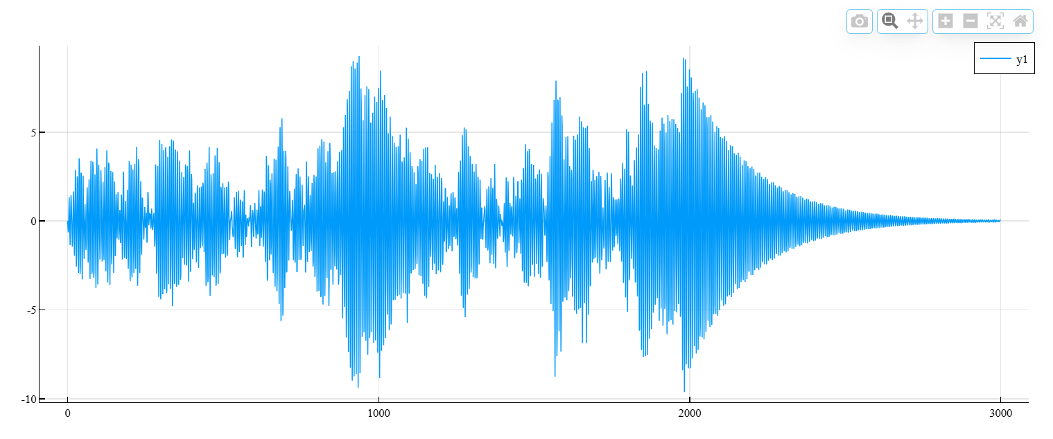
Let’s evaluate the modal frequency response of the system. We use the Hanna window, the length of which is half the length of the measured signals. We indicate that the output signal is the movement of the mass.
wind = hann(Int64.(N/2));
u = vec(u)
frf,f,coh = modalfrf(u',y',Fs,wind,Sensor="dis",out=:data)
The frequency response of a discrete system can be expressed as the Z-transform of the transfer function of the system in the time domain, calculated on the unit circle. Let’s compare the rating modalfrf with a definition.
b,a = ss2tf(A,B,C,D);
ztf,fz = freqz(b,a,2048,Fs);

using Plots

frf_siso = vec(frf[:, 1, 1])
ztf_siso = vec(ztf[:, 1, 1])

plot(f, 20 * log10.(abs.(frf_siso) .+ 1e-12), label="FRF", grid=true)
plot!(fz * Fs, 20 * log10.(abs.(ztf_siso) .+ 1e-12), label="ZTF")
ylims!((-60, 40))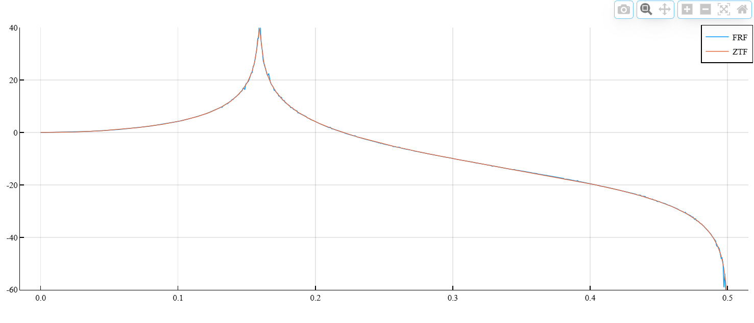
Let’s estimate the natural frequency and attenuation coefficient for a given oscillation mode.
fn,dr,ms,ofrf = modalfit(frf,f,Fs,1,FitMethod="PP",out=:data)

println("fn - ",fn[1])
println("dr - ",dr[1])
fn - 0.15912870854643102
dr - 0.0054516425536509875Let’s compare the natural frequency with , which is the theoretical value for an undamped system.
theo = 1/(2*pi)0.15915494309189535Algorithms
The least squares method for complex exponentials
Details
The least squares method for complex exponentials calculates the impulse response corresponding to each frequency response and approximates the response with a set of complex damped sinusoids using the Prony method. The sampled attenuating sinusoid can be represented as
where
-
— sampling rate;
-
— the frequency of the sine wave;
-
— damping coefficient;
-
and — the amplitude and phase of the sine wave.
Members they are called amplitudes, and — poles. The Proni method expresses a discrete function in the form of a superposition mod (and therefore, amplitudes and poles):
The poles are the roots of a polynomial with coefficients , , …, :
The coefficients are found using an autoregressive model of the form counts from :
To find the poles, the algorithm uses the function roots. Once the poles are known, the frequencies and damping coefficients can be determined by calculating the imaginary and real parts of the logarithms of the poles. The final step is to find the amplitudes and reconstruct the impulse response using
The following simple implementation captures the essence of the procedure:
import EngeeDSP.Functions: hankel, roots

N = 4
L = 2 * N
h = rand(L)
c = -hankel(h[1:N], h[L-N+1:L]) \ h[N+1:L]
x = roots([1; reverse(c)])
V = ComplexF64[x[j]^(i-1) for i in 1:L, j in 1:N]
hrec = V * (V \ h[1:L])
result = sum(h - hrec)
0.006229773214838086 + 9.05157097882403e-17imThe system can also be constructed so that it contains samples from several frequency characteristics, and solved using the least squares method.
Peak extraction method
Details
The peak extraction method assumes that each significant peak in the frequency response corresponds to exactly one eigenmode. It is assumed that near the peak, the system behaves like a damped harmonic oscillator with one degree of freedom.:
where
-
— frequency response;
-
— resonance frequency without damping;
-
— relative damping;
-
— constant damping;
-
— elastic constant;
-
— the mass.
At a given peak located at a point the algorithm takes this peak and a fixed number of points on either side of it, replaces the term with the mass of the dummy variable and calculates modal parameters by solving a system of equations:
Literature
-
Allemang, Randall J., and David L. Brown. Experimental Modal Analysis and Dynamic Component Synthesis, Vol. III: Modal Parameter Estimation. Technical Report AFWAL-TR-87-3069. Air Force Wright Aeronautical Laboratories, Wright-Patterson Air Force Base, OH, December 1987.
-
Brandt, Anders. Noise and Vibration Analysis: Signal Analysis and Experimental Procedures. Chichester, UK: John Wiley & Sons, 2011.
-
Ozdemir, Ahmet Arda, and Suat Gumussoy. Transfer Function Estimation in System Identification Toolbox via Vector Fitting. Proceedings of the 20th World Congress of the International Federation of Automatic Control, Toulouse, France, July 2017.