modalfrf
Frequency characteristics for modal analysis.
| Library |
|
Syntax
Function call
-
frf,f,coh = modalfrf(x,y,fs,window,out=:data)— calculates the matrix of frequency transfer functionsfrfbased on the excitation signalsxand response signalsy, the sampling frequency of which is equal tofs. Output argumentfrfrepresents an estimate calculated using the Welch method with a windowwindowfor windowed signal conversion. Argumentsxandythey must have the same number of rows. IfxoryIf they are matrices, then each column represents one signal.It is assumed that the system response
ycontains acceleration measurements. To calculate frequency characteristics based on displacement or velocity measurements, use the argumentSensor. FunctionmodalfrfIt always outputs frequency characteristics in a dynamic flexibility (sensitivity) format, regardless of the sensor type.
-
frf,f,coh = modalfrf(_,Name,Value,out=:data)— sets additional parameters using arguments like «name-value» for any of the previous syntax options.
-
modalfrf(_,out=:plot)— plots frequency characteristics. The graphs are limited to the first four excitation signals and four response signals.
Arguments
Input arguments
# x — excitation signals
+
vector | the matrix
Details
Excitation signals specified as a vector or matrix.
| Типы данных |
|
# y — response signals
+
vector | the matrix
Details
Response signals specified as a vector or matrix.
| Типы данных |
|
#
fs —
sampling
rate
positive scalar
Details
The sampling frequency in Hz, set as a positive scalar.
| Типы данных |
|
# window — window
+
an integer | vector
Details
A window specified as an integer or vector. Use the argument window to split the signal into segments:
-
If
window— an integer, thenmodalfrfdividesxandyinto segments of lengthwindowand applies a rectangular window of this length to each segment. -
If
window— vector, thenmodalfrfdividesxandyinto segments whose length is equal to the length of the vectorwindow, and applies a window to each segmentwindow.
If the length is x and y it is impossible to accurately divide into an integer number of segments with noverlap with overlapping samples, the signals are truncated accordingly.
Example: hann(N+1) or (1-cos(2*pi*(0:N)'/N))/2 The window is set to be Hannah long N+1.
| Типы данных |
|
# noverlap — number of overlapping counts
+
0 (by default) | a positive integer
Input arguments «name-value»
Specify optional argument pairs as Name,Value, where Name — the name of the argument, and Value — the appropriate value. Type arguments «name-value» they should be placed after the other arguments, but the order of the pairs does not matter. You can specify multiple pairs «name-value».
Use commas to separate the name and value, and Name enclose it in quotation marks, or use an equal sign to separate the name and value, and Name specify it without quotation marks.
Example: modalfrf(x,y,fs,window, "Sensor","vel","Estimator","H1") or modalfrf(x,y,fs,window, Sensor="vel", Estimator="H1") indicates that the input signal consists of speed measurements and is selected as an estimate. "H1".
# Estimator — rating
+
"H1" (by default) | "H2" | "Hv"
Details
The score is set as "H1", "H2" or "Hv":
-
Use
"H1"if the noise does not correlate with the excitation signals. -
Use
"H2"if the noise does not correlate with the response signals. In this case, the number of excitation signals should be equal to the number of response signals. -
Use
"Hv"to minimize the discrepancy between the modeled and estimated response data by minimizing the trace of the error matrix. Value — this is the geometric average of the values and : . The measurement must be single-channel (single-input/single-output, SISO).
# Feedthrough — presence of a gap in the state space model
+
false (default) | true
Details
The presence of bandwidth in the state space model, set as a Boolean value.
| Типы данных |
|
# Measurement — measurement configuration
+
"fixed" (default) | "rovinginput" | "rovingoutput"
Details
Measurement configuration for an equal number of excitation and response channels, specified as "fixed", "rovinginput" or "rovingoutput":
-
Use
"fixed"if the excitation sources and sensors are located at fixed points in the system. Every arousal affects every response. -
Use
"rovinginput"if the measurements are obtained as a result of a movable excitation test (or a movable hammer). One sensor is located in a fixed location of the system. One excitation source is placed at several points and generates one signal from the sensor for each point. Function outputfrf(:,:,i) = modalfrf(x(:,i),y(:,i)). -
Use
"rovingoutput"if the measurements are obtained as a result of a test with a movable sensor. One source of excitation is located in a fixed location of the system. One sensor is placed at several points and responds to one excitation at each point. Function outputfrf(:,i) = modalfrf(x(:,i),y(:,i)).
# Order — the order of the state space model
+
1:10 (by default) | an integer | vector is a string of integers
Details
The order of the state space model, specified as an integer or a vector string of integers. If a vector of integers is specified, the function selects the optimal order value from the specified range.
| Типы данных |
|
# Sensor — sensor type
+
"acc" (default) | "dis" | "vel"
Details
The type of sensor specified as "acc", "vel" or "dis".
-
"acc"— indicates that the system’s response signal is proportional to acceleration; -
"vel"— indicates that the system’s response signal is proportional to the speed; -
"dis"— indicates that the system’s response signal is proportional to the displacement.
Function modalfrf It always outputs the frequency response in a dynamic flexibility (sensitivity) format, regardless of the sensor type.
For an example of using this argument, see Undamped harmonic oscillator.
# out — type of output data
+
:plot (by default) | :data | :all
Details
Type of output data:
-
:plot— the function returns a graph; -
:data— the function returns data; -
:all— the function returns data and a graph.
For this argument, the name and value are separated by an equal sign (=).
|
Output arguments
# frf — frequency characteristics
+
vector | the matrix | array
Details
Frequency characteristics returned as a vector, matrix, or array. Argument frf has a size of on on , where — number of frequency intervals, — the number of response signals, and — the number of excitation signals.
Function modalfrf It always outputs the frequency response in a dynamic flexibility (sensitivity) format, regardless of the sensor type.
# coh — the matrix of multiple coherence
+
the matrix
Details
The multiple coherence matrix returned as a matrix. The matrix coh it has one column for each response signal.
Examples
Undamped harmonic oscillator
Details
Motion of a simple undamped harmonic oscillator with unit mass and elastic constant, sampled with frequency , is described by the transfer function
where the numerator depends on the measured value:
-
moving: ;
-
speed: ;
-
boost: ;
Let’s calculate the frequency response for three possible types of system response sensors. We use the sampling frequency 2 Hz and 30 000 samples of white noise as input data.
import EngeeDSP.Functions: modalfrf, filter,hann
fs = 2
dt = 1/fs
N = 30000
u = randn(N,1)
ydis = filter((1-cos(dt))*[0 1 1],[1 -2*cos(dt) 1],u)
w=hann(Int64.(N/2))

frfd,fd,coh = modalfrf(u,ydis,fs,w,Sensor="dis",out=:data)

yvel = filter(sin(dt)*[0 1 -1],[1 -2*cos(dt) 1],u)
frfv,fv,coh = modalfrf(u,yvel,fs,hann(Int64.(N/2)),Sensor="vel",out=:data)

yacc = filter([1 -(1+cos(dt)) cos(dt)],[1 -2*cos(dt) 1],u)
frfa,fa,coh = modalfrf(u,yacc,fs,hann(Int64.(N/2)),Sensor="acc",out=:data)

frfd_vec = frfd[:]
frfv_vec = frfv[:]
frfa_vec = frfa[:]

plot(fd, abs.(frfd_vec), xscale=:log10, yscale=:log10, label="dis", grid=true)
plot!(fv, abs.(frfv_vec), xscale=:log10, yscale=:log10, label="vel", grid=true)
plot!(fa, abs.(frfa_vec), xscale=:log10, yscale=:log10, label="acc", grid=true)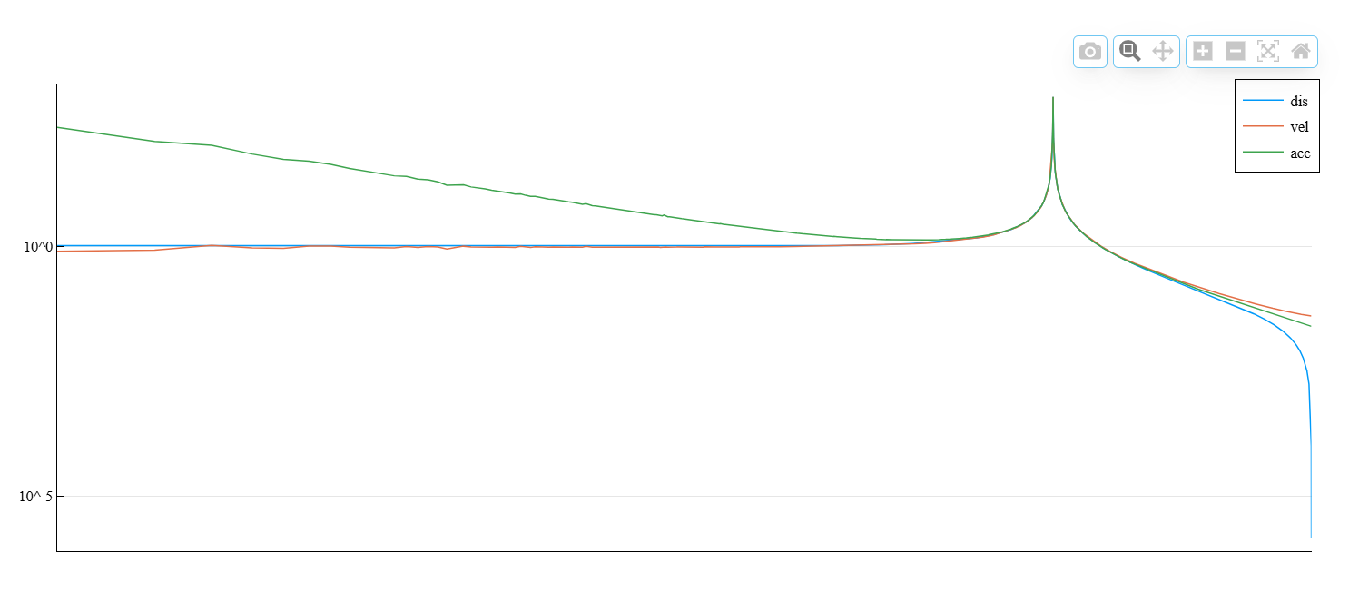
In all cases, the generated frequency response has a format corresponding to the displacement. The velocity and acceleration measurements are, respectively, the first and second time derivatives of the displacement measurements. The frequency characteristics are equivalent in the range around the natural frequency of the system. Away from the natural frequency, the frequency characteristics vary.
Frequency response of a single-channel system
Details
Let’s evaluate the frequency response of a simple single-channel (single-input/single-output, SISO) system and compare it with the definition.
A one-dimensional discrete oscillatory system consists of a single mass in kg, attached to the wall by a spring with constant elasticity N/M. The sensor registers the mass displacement with frequency Hz. The damper prevents the movement of the mass, exerting a force proportional to the velocity on it, with a constant damping kg/sec.

Generate 3000 time counts. Let’s define the sampling interval .
import EngeeDSP.Functions: modalfit, randn, modalfrf, hann, ss2tf, freqz

Fs = 1
dt = 1/Fs
N = 3000
t = dt*(0:N-1)
b = 0.01
The system can be described using a state space model.:
where is the state vector, and — respectively, the displacement and velocity of the mass, — the driving force, and — measured output signal. State space matrices:
where — the identity matrix , and the matrices of the state space in continuous time have the form:
Ac = [0 1; -1 -b]
A = exp(Ac * dt)

Bc = [0; 1]
B = Ac \ (A - [1 0; 0 1]) * Bc

C = [1 0]
D = 0
During the first 2000 For a few seconds, the mass is set in motion by random action, and then it is allowed to return to rest. We use the state space model to calculate the time evolution of the system, starting from the zero initial state. Let’s plot the mass displacement as a function of time.
using Random

Random.seed!(1234)
u = randn(1,N) / 2
u[2001:end] .= 0

y = zeros(N)
x = [0.0; 0.0]

for k in 1:N
    y[k] = (C * x)[1] + D * u[k]
    x = A * x + B * u[k]
end


t = dt * (0:N-1)
plot(t, y, grid=true)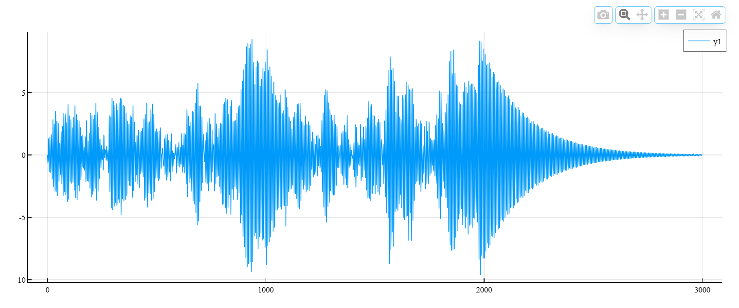
Let’s evaluate the modal frequency response of the system. We use the Hanna window, the length of which is half the length of the measured signals. We indicate that the output signal is the movement of the mass.
wind = hann(Int64.(N/2));
u = vec(u)
frf,f,coh = modalfrf(u',y',Fs,wind,Sensor="dis",out=:data)
The frequency response of a discrete system can be expressed as the Z-transform of the transfer function of the system in the time domain, calculated on the unit circle. Let’s compare the rating modalfrf with a definition.
b,a = ss2tf(A,B,C,D);
ztf,fz = freqz(b,a,2048,Fs);

using Plots

frf_siso = vec(frf[:, 1, 1])
ztf_siso = vec(ztf[:, 1, 1])

plot(f, 20 * log10.(abs.(frf_siso) .+ 1e-12), label="FRF", grid=true)
plot!(fz * Fs, 20 * log10.(abs.(ztf_siso) .+ 1e-12), label="ZTF")
ylims!((-60, 40))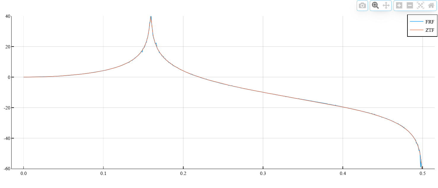
Let’s estimate the natural frequency and attenuation coefficient for a given oscillation mode.
fn,dr,ms,ofrf = modalfit(frf,f,Fs,1,FitMethod="PP",out=:data)

println("fn - ",fn[1])
println("dr - ",dr[1])
fn - 0.15912870854643102
dr - 0.0054516425536509875Let’s compare the natural frequency with , which is the theoretical value for an undamped system.
theo = 1/(2*pi)0.15915494309189535Literature
-
Dynamic Stiffness, Compliance, Mobility, and more Siemens, last modified 2019, https://community.sw.siemens.com/s/article/dynamic-stiffness-compliance-mobility-and-more.
-
Brandt, Anders. Noise and Vibration Analysis: Signal Analysis and Experimental Procedures. Chichester, UK: John Wiley & Sons, 2011.
-
Irvine, Tom. An Introduction to Frequency Response Functions Vibrationdata, 2000, https://vibrationdata.com/tutorials2/frf.pdf.
-
Vold, Havard, John Crowley, and G. Thomas Rocklin. New Ways of Estimating Frequency Response Functions. Sound and Vibration. Vol. 18, November 1984, pp. 34–38.