rainflow
Fatigue characteristics analysis by the method «Rain».
| Library |
|
Syntax
Arguments
Input arguments
x —
the pattern of load changes over time
+
vector
Details
The pattern of load changes over time, set as a vector. Argument x must contain the final values.
| Типы данных |
|
fs —
sampling rate
+
scalar
Details
The sampling frequency, set as a positive real scalar.
| Типы данных |
|
t —
time values
+
vector
Details
Time values set as a vector representing the time interval between counts.
| Типы данных |
|
Input arguments «name-value»
Specify optional argument pairs as Name=Value, where Name — the name of the argument, and Value — the appropriate value. Type arguments «name-value» they must be placed after other arguments.
out —
type of output data
+
:data (by default) | :plot
Details
Type of output data:
-
:data— the function returns data; -
:plot— the function returns a graph.
Output arguments
c —
number of cycles
+
the matrix
Details
Data on the number of cycles returned as a matrix. The matrix c It contains information about cycles in the following columns: quantity, load ranges, average load values, cycle start indexes and cycle end indexes. For an example, see Algorithms. If the sampling frequency, time interval, or time value vector is specified, then the last two columns of the matrix c they contain the initial and final cycle duration.
rm —
the matrix of rain flows
+
the matrix
Details
The matrix of rain flows. Lines rm they correspond to the load range of the cycles, and the columns correspond to the average load value of the cycle.
idx —
linear indexes of turning points
+
vector
Details
Linear indexes of the turning points returned as a vector.
Examples
Counting cycles of identified turning points
Details
We will generate a set of extremes that simulate changes in the direction of the load. Let’s plot the data graph.
X = [-2, 1, -3, 5, -1, 3, -4, 4, -2]


plot(X, xlabel="Sample Index", ylabel="Stress")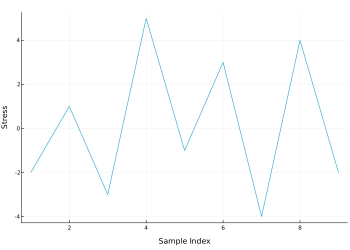
Let’s calculate the number of cycles for this data. We indicate that the input data consists of already identified extremes.
import EngeeDSP.Functions: rainflow


C, hist, edges = rainflow(X, "ext")
Let’s plot a histogram of the number of cycles depending on the voltage load range.
counts = sum(hist, dims=2)[:]


bin_centers = (edges[1:end-1] + edges[2:end]) / 2

bar(bin_centers, counts, xlabel="Stress Range", ylabel="Cycle Counts")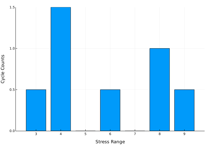
Algorithms
Fatigue performance analysis examines how damage accumulates in an object subject to cyclic stress changes. The number of cycles required to destroy an object depends on the amplitude of the cycle. The broadband input excitation contains cycles of various amplitudes, and the presence of hysteresis in the object leads to the fact that some cycles are fully or partially embedded in others. _ mEthod «Rain»_ estimates the number of load change cycles as a function of the cycle amplitude.
First, the function rainflow converts the load change pattern into a sequence of _ rotating points_. Turning points are local minima and maxima at which the load changes sign. The function counts cycles by considering a moving reference point of the sequence Z and a moving ordered subset of three points with the following characteristics:
-
The first and second points are collectively called Y.
-
The second and third points are collectively called X.
-
At both points, X and Y points are sorted by time from earlier to later, but are not necessarily ordered in the sequence of turning points.
-
The load range of values X, denoted as r(X), is the absolute value of the difference between the amplitude of the first point and the amplitude of the second point. The definition of r(Y) is similar.
The algorithm of the function rainflow it looks like this:
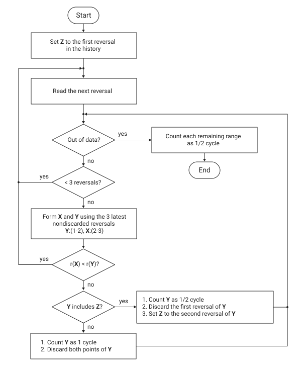
At the end, the function collects data on various cycles and half-cycles and makes a table of their load ranges, average load values, and start and end points. This information can then be used to build a cycle histogram.
Consider the following sequence of turning points:
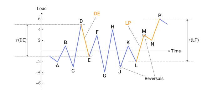
| Step | Z | Turning points | Three turning points? | Y | r(Y) | X | r(X) | r(X) < r(Y)? | Z in Y? | Actions |
|---|---|---|---|---|---|---|---|---|---|---|
1 |
A |
A, B, C |
Yes |
AB |
3 |
BC |
4 |
No |
Yes |
|
2 |
B |
B, C |
No |
— |
— |
— |
— |
— |
— |
Read D |
3 |
B |
B, C, D |
Yes |
BC |
4 |
CD |
8 |
No |
Yes |
|
4 |
C |
C, D |
No |
— |
— |
— |
— |
— |
— |
Read E |
5 |
C |
C, D, E |
Yes |
CD |
8 |
DE |
6 |
Yes |
— |
Read F |
6 |
C |
C, D, E, F |
Yes |
DE |
6 |
EF |
4 |
Yes |
— |
Read G |
7 |
C |
C, D, E, F, G |
Yes |
EF |
4 |
FG |
7 |
No |
No |
|
8 |
C |
C, D, G |
Yes |
CD |
8 |
DG |
9 |
No |
Yes |
|
9 |
D |
D, G |
No |
— |
— |
— |
— |
— |
— |
Read H |
10 |
D |
D, G, H |
Yes |
DG |
9 |
GH |
8 |
Yes |
— |
Read J |
11 |
D |
D, G, H, J |
Yes |
GH |
8 |
HJ |
7 |
Yes |
— |
Read K |
12 |
D |
D, G, H, J, K |
Yes |
HJ |
7 |
JK |
4 |
Yes |
— |
Read L |
13 |
D |
D, G, H, J, K, L |
Yes |
JK |
4 |
KL |
3 |
Yes |
— |
Read M |
14 |
D |
D, G, H, J, K, L, M |
Yes |
KL |
3 |
LM |
5 |
No |
No |
|
15 |
D |
D, G, H, J, M |
Yes |
HJ |
7 |
JM |
5 |
Yes |
— |
Read N |
16 |
D |
D, G, H, J, M, N |
Yes |
JM |
5 |
MN |
1 |
Yes |
— |
Read P |
17 |
D |
D, G, H, J, M, N, P |
Yes |
MN |
1 |
NP |
4 |
No |
No |
|
18 |
D |
D, G, H, J, P |
Yes |
HJ |
7 |
JP |
9 |
No |
No |
|
19 |
D |
D, G, P |
Yes |
DG |
9 |
GP |
10 |
No |
Yes |
|
20 |
G |
G, P |
There is no data |
— |
— |
— |
— |
— |
— |
Count GP as half a cycle |
Now let’s collect the results.
| Number of cycles | Load range | Average load value | Beginning | The end |
|---|---|---|---|---|
1/2 |
3 |
−0.5 |
A |
B |
1/2 |
4 |
−1 |
B |
C |
1 |
4 |
1 |
E |
F |
1/2 |
8 |
1 |
C |
D |
1 |
3 |
−0.5 |
K |
L |
1 |
1 |
2.5 |
M |
N |
1 |
7 |
0.5 |
H |
J |
1/2 |
9 |
0.5 |
D |
G |
1/2 |
10 |
1 |
G |
P |
Let’s compare this with the result of applying the algorithm of the function rainflow for a given sequence:
import EngeeDSP.Functions: rainflow


q = rainflow([-2 1 -3 5 -1 3 -4 4 -3 1 -2 3 2 6])[1]
9×5 Matrix{Float64}:
0.5 3.0 -0.5 1.0 2.0
0.5 4.0 -1.0 2.0 3.0
1.0 4.0 1.0 5.0 6.0
0.5 8.0 1.0 3.0 4.0
1.0 3.0 -0.5 10.0 11.0
1.0 1.0 2.5 12.0 13.0
1.0 7.0 0.5 8.0 9.0
0.5 9.0 0.5 4.0 7.0
0.5 10.0 1.0 7.0 14.0Literature
-
ASTM E1049-85(2017), Standard Practices for Cycle Counting in Fatigue Analysis. West Conshohocken, PA: ASTM International, 2017, https://www.astm.org/e1049-85r17.html.