tachorpm
Extracting the speed signal from the pulse signal of the tachometer.
| Library |
|
Syntax
Function call
-
tachorpm(___,out=:plot)— plots the calculated speed signal and the tachometer signal with detected pulses.
Arguments
Input arguments
# x — tachometer pulse signal
+
vector
Details
The pulse signal of the tachometer, set as a row vector or column vector.
#
Fs — sampling
rate
scalar
Details
The sampling frequency in Hz, set as a positive scalar.
Input arguments «name-value»
Specify optional argument pairs as Name,Value, where Name — the name of the argument, and Value — the appropriate value. Type arguments «name-value» they should be placed after the other arguments, but the order of the pairs does not matter. You can specify multiple pairs «name-value».
Use commas to separate the name and value, and Name enclose it in quotation marks, or use an equal sign to separate the name and value, and Name specify it without quotation marks.
Example: rpm = tachorpm(x, Fs, "PulsesPerRev", 3, "OutputFs", 1e3) or rpm = tachorpm(x, Fs, PulsesPerRev = 3, OutputFs = 1e3) indicates that there are three tachometer pulses per revolution, and the returned speed signal must be sampled with the frequency 1 kHz.
# PulsesPerRev — the number of tachometer pulses per revolution
+
1 (default) | scalar
Details
The number of tachometer pulses per revolution, set as a real scalar.
# StateLevels — state levels for pulse identification
+
two-element vector
Details
The state levels used to identify the pulses are specified as a two-element real vector.
The first element of the vector corresponds to a low state level, and the second element corresponds to a high state level. Select the state levels so that each pulse edge intersects both levels within 10%. If this argument is omitted, the function tachorpm automatically calculates levels using the histogram method, which is used in the function statelevels.
# OutputFs is the sampling rate of the output signal
+
Fs (default) | scalar
Details
The sampling frequency of the output signal, set as a real scalar.
# FitType — approximation method
+
"smooth" (by default) | "linear"
Details
An approximation method defined by one of the following values:
-
"smooth"— approximation of the rotation frequency values on pulses by the B-spline least squares method; -
"linear"— linear interpolation between the values of the rotational speed on the pulses.
# FitPoints — B-spline split points
+
10 (default) | scalar
Details
The number of B-spline split points, given as a real scalar.
The number of split points determines the ratio between the smoothness of the curve and the proximity to the original data. Too many points can lead to overfitting. Function tachorpm ignores this argument if the argument FitType assigned value "linear".
# out — type of output data
+
:data (default) | :plot
Details
Type of output data:
-
:data— the function returns data; -
:plot— the function returns a graph.
For this argument, the name and value are separated by an equal sign (=).
|
Examples
Extracting the rotation speed signal
Details
Calculate the speed signal from a given tachometer signal x with sampling rate fs = 300 Hz using the function tachorpm using the default values. Visualize the result.
import EngeeDSP.Functions: tachorpm

x = [0.0123687231949916 0.012929057487293 0.00370767140060606 -0.0127867455844306 0.0207798656342499 0.0149300342450755 -0.00257492375812022 0.0101513511337194 0.000221061466986783 0.0134107717285896 -0.00032638837471522 0.00264658439791083 -0.0143828404346631 0.00112171981189251 -0.00532699201156813 0.00481279396579837 -0.0132256568321587 -0.0134236371554794 0.0135267695369469 -0.0118623459528275 0.325732263905399 1.00599505357105 0.340546043324391 -0.00341132970925447 0.0117886531893246 0.00907790735669179 -0.00937073341626731 -0.00662456631297685 0.0105554596805873 -0.0123222191616032 0.0077712008280042 0.00148460369048622 0.0201243480405002 -0.0129239931688391 0.0104841421024252 0.000807308563014007 0.00345245561139732 -0.015389951968041 0.00495555611861497 0.00568242650216338 0.0170058773587523 -0.0117929075880624 -0.0146033669978636 -0.0051745915436029 0.00854647319250477 -0.00379598313133096 -0.0206009704447754 0.000229447701471211 -0.00144866010581576 0.345045319139853 1.00476947651622 0.331390666995008 -0.00600030925764606 -0.00300313598346054 0.0151081065255403 -0.0165624038809835 -0.00310657525290631 0.00355618442778826 -0.003233055312466 -0.000536419894749568 0.0118683350987834 -0.00527313070208185 0.00242228713889516 -0.00831979062711107 -0.00758341618554786 0.000557701568753797 -0.0230442758076321 -0.00818176566521673 0.00604900635681608 0.00383724098379988 -0.00750622368719906 0.00434557877734846 0.00592057925766131 0.0104374669060945 -0.00950168323445638 -0.0205776712008571 0.0132700375010382 0.333462756069495 0.993194264295042 0.348408806121347 -0.00316601639928196 -0.00101667512862816 -0.00382150728939923 0.0152468531360328 -0.0010492485728069 -0.00774816000072779 0.00622307134169297 0.000616728048525806 0.00634886505365873 -0.00587222466780974 -0.0189104172908645 -0.00376414390709292 0.0167857677307849 -0.0042247141613658 0.00933825757733899 0.0143681310724238 -0.0134713439956526 -0.00048606420547968 0.0236970319802929 0.0110583657512326 0.00228990015305506 0.0255721576969559 0.00258238252255179 -0.0167654516834903 0.00309754955281608 0.00744000441780851 0.335480905533579 1.00150524731801 0.335745888523375 -0.00557110546579485 -0.0163241712211035 0.00673765946037728 -0.00015172163281829 0.0113408931166143 -0.0177446636830673 -0.0091775246687951 0.0110984007355662 0.0107296867994391 0.00918353531652778 -0.00333171376524465 0.00542823067992952 0.00354918556632447 0.0154287839679142 0.00159700927345757 -0.00573722994539428 0.00314638503912775 -0.0077018245520029 0.0144599109872083 0.0111154321086023 0.00837498029881252 -0.00948133925972314 0.00532257142640029 -0.011159181487983 0.000248121953946674 0.331178572808174 0.991000860795657 0.326420065862715 0.000921678486817408 -0.00333955488833592 0.00606157716107364 0.0129381693199957 -0.00234247267422009 -0.00371035908729699 0.00353054237205674 0.0085110347237396 0.00351119854479667 -0.00512430455330845 0.0107386241915759 0.00683852268033496 0.00131145852379954 0.000551611363298636 -0.000803285552740011 0.0099935466964052 -0.00424058690118701 0.00743887948504606 0.00463566203470817 0.00136562009929537 0.0184269680957754 0.00594542876143403 0.000689702792290508 0.00232558275816203 0.0140348702462655 0.360008383489613 0.999152430331844 0.326733314752749 -0.00821514846848881 -0.00814352565876977 0.0158403151517346 0.0014732130402467 0.00693351776343055 -0.00627647127347142 0.00773393394074708 0.00022463111837903 -0.00641877967191403 -0.0209217954508951 0.00336674902268624 -0.0132280971595629 -0.0114786371412884 2.98481085063913e-5 -0.00945485177461916 -0.0025776880504647 -0.00661003592538187 -0.0233662670350878 -0.00352356496203137 -0.00564348956146911 -0.00466679014527461 0.00840927871030486 -0.012589910559448 -0.00154211740840474 0.0116766647202132 0.330616984620313 0.988276509918218 0.337328557005741 0.0241234274826587 -0.0162929425209768 0.014181901621891 -0.00759005617739814 -0.00161510061123031 0.00782476271265081 -0.00437968205667631 0.00171351538942357 0.00804994623055304 -0.00253826021482742 0.0110511649865298 -0.00391978035790193 -0.00494413324966295 0.00117858622500355 -0.0124152082285886 -0.0104568387612462 -0.00844150046071535 -0.0034994947575161 0.00385941374048937 0.0156137751117932 -0.0178454698410544 -0.0086787080312056 -0.0047404573950102 -0.011366072514341 0.0016957651970677 0.337682137573958 0.999425710026516 0.315715336864508 0.0173149523070065 0.0116445190653724 0.00729016999231267 -0.0195000311320162 -0.00756961838882072 -0.0210825300793485 0.00138295314058436 0.0117733622506946 -0.00332344700420788 -0.0200889500858694 0.010625422638581 -0.00250168933892938 0.00209981326417487 0.00378172884909814 0.00850329920497805 0.0264397723452991 0.0126414249854762 -0.000458795116066035 0.00298344313531912 0.0106978581459031 -0.0048432421491483 0.00235249886061713 -0.00190886955902538 0.0173730545858268 -0.00483131414020375 0.353267903433487 0.998645915272625 0.344835010377289 -0.000942362017288848 0.00836968855050359 0.0156717506500162 -0.00619834776797133 -0.0139444407440782 -0.00221979385523925 0.00882095578165526 -0.00948526111985494 0.0151122077825191 0.00918426909732982 0.000552585712473191 0.00860883019975887 0.00502474107107943 0.00861659557782132 0.0124068636591337 -0.00863533891327363 0.00782365632526516 0.00490109505311577 0.00989613559341397 -0.00446256579762467 0.00096029242376651 -0.00744455497189824 -0.00260690838044167 -0.00969344424080115 0.32598727408206 0.987285534385729 0.338510537759917 -0.0130393845866332 -0.00756763496329479 -0.00425048883449127 0.000337674314884639 0.0248261971077493 -0.00846513468206622 -0.00789126742733859 0.0117862902231557 -0.011068462545708 0.0173771648346555 0.00336649928185011 0.0168910911578464 -0.00798431302611711 0.00422260766767306 0.00139800916411764 0.00195622470993301 0.00241022965721666 -0.00372529709577477 0.000361373598859211 0.013127222849596 -0.00288138336621927 0.00550808964195426 -0.00274428182860599 0.000469532594057926]
fs = 300

tachorpm(x, fs, out = :plot)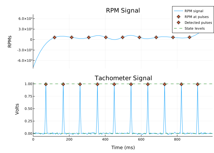
Algorithms
Function tachorpm performs the following actions:
-
Using the function
statelevelsdetects the low and high levels of the tachometer signal. -
Using the functions
risetimeandfalltimedetermines the start and end time of each pulse, and then averages these values to find the time point corresponding to each pulse.Function
tachorpmdetects rising and falling edges independently and in pairs, without guessing which edge appears first in the tachometer signal. If the pulse starts in the middle of the cycle, the function may not match the edges correctly. For example, this is possible when a sequence of fronts corresponds to a high level. «rising — falling — rising», and the signal starts with a falling edge. In order for the function to correctly calculate the rotation speed in such cases, trim the tachometer signal so that its first edge is rising and indicates the beginning of the full pulse cycle. -
Using the function
diffdetermines the time intervals between the pulse centers and calculates the rotation frequency values in the middle of the intervals using the formula . -
If the argument
FitTypeassigned value"smooth", performs the least squares approximation using the functionspline. If the argumentFitTypeassigned value"linear", performs linear interpolation using the functioninterp1.
Literature
-
Brandt, Anders. Noise and Vibration Analysis: Signal Analysis and Experimental Procedures. Chichester, UK: John Wiley & Sons, 2011.
-
Vold, Håvard, and Jan Leuridan. «High Resolution Order Tracking at Extreme Slew Rates Using Kalman Tracking Filters.» Shock and Vibration. Vol. 2, 1995, pp. 507–515.