Critical gas outflow mode
Let's build a model of the effects that occur in a pipe when the gas flow becomes critical.
Description of the phenomenon
Library blocks for modeling gas processes, such as Local Restriction (G), Variable Local Restriction (G), or Pipe (G), support modeling critical gas flow.
Critical flow occurs when the flow velocity in a certain section reaches the local speed of sound. At a critical flow, the velocity in this section can no longer increase. However, the mass flow rate can continue to increase if the gas density is increased. This can be achieved, for example, by increasing the pressure in front of the critical flow point.
We will observe the effect of the critical flow in the pipe. The effect will be that the mass flow rate in the block modeling the pipe will depend entirely on the pressure and temperature in front of the block. When a critical flow condition is formed and as long as it persists, this supercritical mass flow rate will no longer depend on the pressure value in the space after the block.
Description of the model
We will demonstrate the effect of the critical flow on the following model. In it, the Ramp block has a slope of 0.005 MPa (5e3 Pa), while the rise begins at a time of 10 s. For the remaining blocks, all parameters have default values. The total calculation time is 50 seconds.
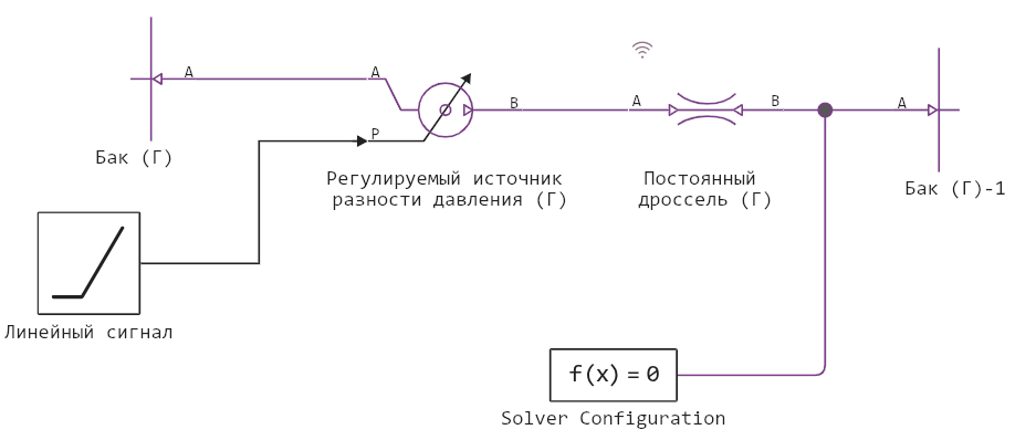
When starting the model, the pressure on port A of the block is Permanent throttle (G) increases linearly from atmospheric pressure, starting at 10 seconds. The pressure at port B is fixed at atmospheric pressure.
model_name = "choked_flow_demo";
model_name in [m.name for m in engee.get_all_models()] ? engee.open(model_name) : engee.load( "$(@__DIR__)/$(model_name).engee");
res = engee.run( model_name );
The graph shows the result of calculating the process around the block Permanent throttle (G). The Mach number in the constriction (Mach) reaches a value of 1 at about 20 seconds, which indicates the occurrence of a critical flow.
mdot_a = res["Permanent throttle (D).mdot_a"];
Mach = res["Permanent throttle (G).Mach"];

plot(Mach.time, Mach.value, lw=2, title="Throttle Mach Speed (Mach)",
     legend=false, titlefont=font(11))
plot(mdot_a.time, mdot_a.value, lw=2, title="Mass flow through throttle (mdot_a)",
     legend=false, titlefont=font(11))
The mass flow rate (mdot_A) before the critical mode occurs varies quadratically with increasing pressure drop. However, after reaching the critical mode, the mass flow rate becomes linear, * since the subcritical mass flow rate depends only on the pressure and temperature before the constriction, and the pressure in front of the block increases linearly*.
Simulation with a compressor
The fact that the subcritical mass flow rate depends only on the upstream conditions may lead to incompatibility with the Mass Flow Rate Source (G) block. or Controlled Mass Flow Rate Source (G), connected after the (downstream) block with critical flow.
General rule: if a critical flow is possible in the model, use pressure sources, and not****mass flow sources.
If the model contains mass flow source blocks and the simulation fails, analyze the values of the Mach number in different structural elements, especially chokes and pipes.
If an error occurs when the Mach number is reached = 1, then it is likely that the mass flow source located after the critical flow unit is trying to set the flow rate above the possible value for critical flow.
Conclusion
We have clearly shown how the critical flow limits the maximum gas flow and makes it depend only on the inlet pressure and temperature — this is a key effect that cannot be ignored when calculating pipelines and throttling elements.
Modeling of such systems is critically important, because without it, you can mistakenly set an unrealistic flow rate or fail to take into account abrupt changes in flow parameters, which leads to design errors, equipment breakdowns, or even emergencies.