Turbojet engine (system model)
When creating a complex system, models of reduced accuracy are often needed, which allow you to display the complex dynamics of the target product with the correct scale. Even if later it is planned to develop a more specific model of each node of the system, the presence of high-level blocks in the library is extremely important to speed up design.
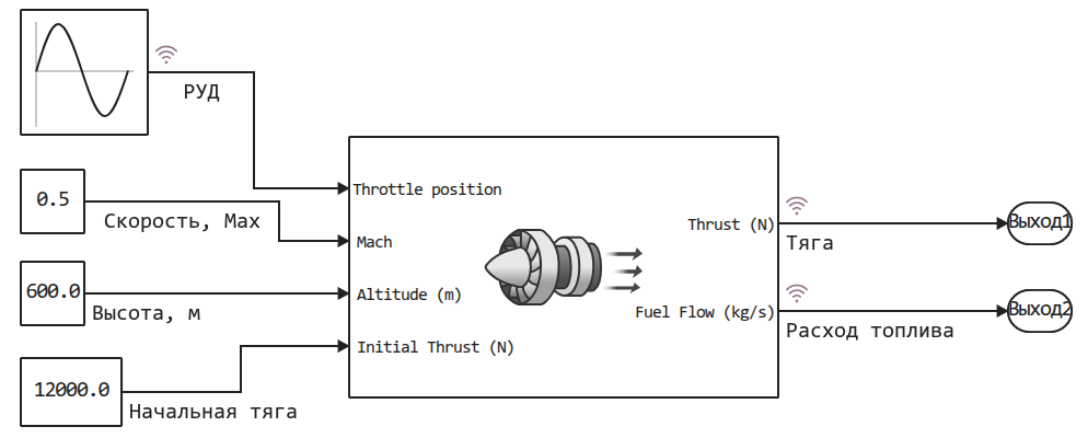
In this example, we will study the use of the "Turbojet Engine" unit and interpret the calculation results.
Block Restrictions
The Turbojet engine unit has only 4 inputs and 4 parameters. One can imagine that a more accurate model will have many more, but in this example we are considering the most high-level of the available GTD models.
To study the internal structure of such a model, we recommend that you pay attention to a more detailed example called "Modeling of a small-scale gas turbine engine".
The main block that this project demonstrates contains a "directional" model with a closed and well-established control system.
This model works like an algorithm, it will not have instability, spurious physical effects, all control circuits are debugged and closed.
To assemble a test bench or at least a more detailed model, it would be necessary to refer to the above-mentioned example or to the blocks of physical modeling. The model based on "acausal" physical blocks will allow us to observe many interesting phenomena (the influence of nozzle dynamics, bypasses, air quality studies, surging and itching, flame disruption, etc.).
However, since they try to minimize the impact of any harmful processes during the design of ACS, this unit is perfectly suitable for the role of a model of a finished product.
Launching a turbojet engine model
Let's run the model to study the results:
model = engee.open("$(@__DIR__)/turbofan_engine_system.engee")
data = engee.run( model )
Let's turn to the variables from the structure data to build multiple graphs:
t = data["ORE"].time
руд = data["ORE"].value
расход = data["Fuel consumption"].value
тяга = data["Thrust"].value

plot(plot(руд, тяга, lw=2, title="Connection of ores and thrust of the gas turbine engine", xlabel="ORE", ylabel="Thrust of the gas turbine engine, N"),
     plot(руд, расход, lw=2, c=2, title = "The relationship between ORES and fuel consumption", xlabel="ORE", ylabel="Fuel consumption, kg/s"),
     legend=false, titlefont=font(12))
Conclusion
The model allowed us to observe the operation cycle of the gas turbine engine during slow movement of ores (a sine wave with a period of 0.1 rad/s) at an altitude of 600 m and at a speed of 0.5 Max. Ore management was carried out in the range from 0 to 1, which is not a realistic scenario for testing a gas turbine engine, but it shows the dynamics of the model well.
By varying the properties of this model and the input parameters, we can observe the effect on integral indicators without spending time on insignificant internal parameters.