Modeling of the Dzhanibekov effect

This example will show a simulation of the Dzhanibekov effect, an unstable rotation of a rigid body around the average axis of inertia. The model demonstrates how a small perturbation during rotation around an intermediate axis leads to a periodic "flip" of an object in space.

The Dzhanibekov effect is manifested when an asymmetric rigid body rotates around an axis with an intermediate moment of inertia. According to the intermediate axis theorem, such rotation is unstable - the slightest disturbance leads to a periodic "flip" of the object.

Occurrence condition: i₁ < i₂ < i₃, where i₂ is the moment of inertia relative to the median axis.

Initial disturbance: .

Model diagram:

To implement the rotation model in this example, the Engee Function block is used, in which, using the code, the Euler equations for free rotation were implemented.:

This section also describes the kinematics of quaternions.:

States are supplied to the input of the block integrals of derivatives of quaternions and angular velocities calculated in the block Integration with the following device:

Using bus blocks, the signals are compiled for future use. From Bus 3, the signal goes to the block, in which the bus is converted into a vector and then fed to the input of the block Transformation of a quaternion into a rotation matrix.

Defining the function to load and run the model:

function start_model_engee()
    try
        engee.close("dzhanibekov_effect", force=true) # closing the model
        catch err # if there is no model to close and engee.close() is not executed, it will be loaded after catch.
            m = engee.load("$(@__DIR__)/dzhanibekov_effect.engee") # loading the model
        end;

    try
        engee.run(m) # launching the model
        catch err # if the model is not loaded and engee.run() is not executed, the bottom two lines after catch will be executed.
            m = engee.load("$(@__DIR__)/dzhanibekov_effect.engee") # loading the model
            engee.run(m) # launching the model
        end
end

start_model_engee (generic function with 1 method)

Running the simulation

start_model_engee();

Output data to a separate variable:

result = collect(simout["dzhanibekov_effect/Преобразование кватерниона
 в матрицу поворота.DCM"]);

Output of data into separate variables for their analysis and visualization:

time_ = result[:,1]
R_hist = result[:,2];

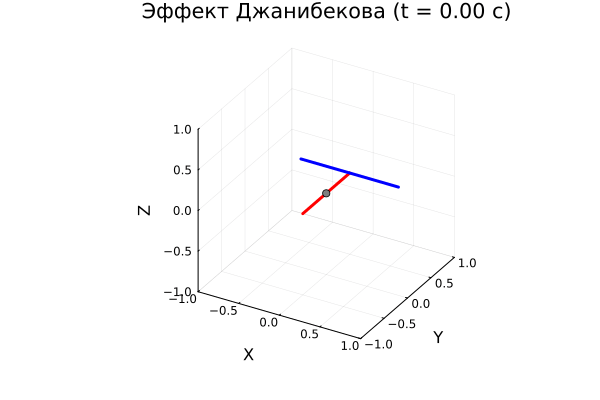
Defining a function to create a T-shaped geometric shape:

function create_t_figure()
    vertical = [[0, 0], [-0.5, 0.5], [0, 0]]
    horizontal = [[-0.6, 0.6], [0.5, 0.5], [0, 0]]
    return (vertical, horizontal)
end

create_t_figure (generic function with 1 method)

Defining a function to create an animation of body movement:

using Printf
function create_djanibekov_animation_plots(R_hist, time_)
    gr()
    # Creating a T-shape
    t_figure = create_t_figure()
    vertical, horizontal = t_figure
    
    # A function for converting points using a rotation matrix
    function rotate_points(points, R)
        x, y, z = points
        n = length(x)
        rotated = zeros(3, n)
        for i in 1:n
            rotated[:, i] = R * [x[i], y[i], z[i]]
        end
        return rotated[1, :], rotated[2, :], rotated[3, :]
    end
    
    # Creating an animation
    anim = @animate for i in 1:40:length(R_hist)
        R = R_hist[i]
        
        # Applying rotation to the shape
        v_rot = rotate_points(vertical, R)
        h_rot = rotate_points(horizontal, R)
        gr()
        # Creating a 3D graph
        p = plot3d(
            v_rot..., 
            linewidth=3,
            linecolor=:red,
            label="",
            xlim=(-1, 1),
            ylim=(-1, 1),
            zlim=(-1, 1),
            title="The Dzhanibekov effect (t = $(@sprintf("%.2f", time_[i])) c)",
            xlabel="X",
            ylabel="Y",
            zlabel="Z",
            aspect_ratio=:equal,
            camera=(30, 30)
        )
        
        plot3d!(
            h_rot...,
            linewidth=3,
            linecolor=:blue,
            label=""
        )
        
        # Adding a sphere in the center
        scatter3d!([0], [0], [0], markersize=4, markercolor=:gray, label="")
    end
    
    # Saving the animation to GIF
    output_path = "djanibekov_effect_plots.gif"
    
    println("Animation saved to a file: ", output_path)
    return gif(anim, output_path, fps=25)
end

create_djanibekov_animation_plots (generic function with 1 method)

Creating and visualizing body movement animations:

anim = create_djanibekov_animation_plots(R_hist, time_)

Анимация сохранена в файл: djanibekov_effect_plots.gif

[ Info: Saved animation to /user/djanibekov_effect_plots.gif

w1 = collect(simout["dzhanibekov_effect/Integration.w₁"])
w2 = collect(simout["dzhanibekov_effect/Integration.w₂"])
w3 = collect(simout["dzhanibekov_effect/Integration.w₃"]);

plotlyjs()
plot(w1[:, 1], w1[:, 2], label="Angular velocity around the X-axis", lw=2)
plot!(w2[:, 1], w2[:, 2], label="Angular velocity around the Y axis", lw=2)
plot!(w3[:, 1], w3[:, 2], label="Angular velocity around the Z axis", lw=2)

The flip can be tracked on the graph by changing the sign of the angular velocity around the Y axis, this happens every 4 seconds.

Conclusions:

In this example, a model of the Dzhanibekov effect was demonstrated. The model can be modified and used in various fields for guidance tasks, target tracking, and for manipulator orientation control.