Determination of the parameters of a permanent magnet synchronous motor (PMSM) on an experimental stand
When working with real engines, it often happens that not all the necessary parameters are specified in the technical documentation. This example shows how to determine the counter-EMF coefficient and the torque constant of a permanent magnet synchronous motor (PMSM) if its flow coupling is unknown.
Imagine that we have a real motor operating in generator mode, at the terminals of which the voltage can be measured. We will rotate its shaft with angular velocity:
angular_velocity = 5; # glad/with
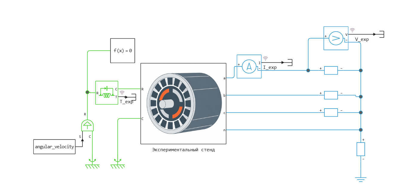
The experimental stand is presented in the model PMSMParameterization.engee a masked subsystem.
As with real experimental measurements, the voltage signal is noisy.
The following is a model based on the PMSM block (library Physical Modeling/Electricity/Electric machines/With permanent magnets).
We will define the missing parameters of the PMSM block in this example.
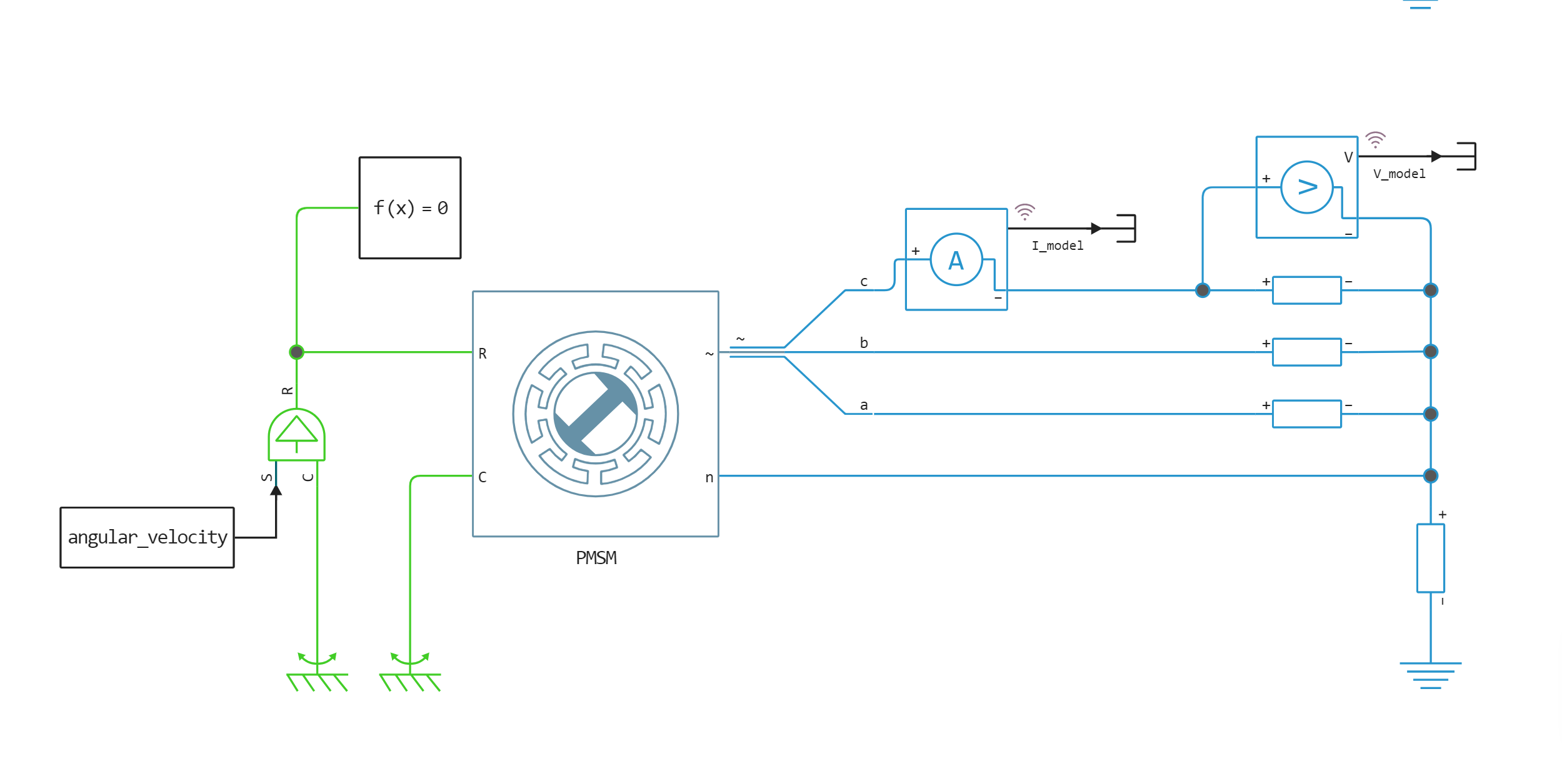
In the unit settings, you can select the method ** for Parameterizing the magnetic flux of permanent magnets**. You can ask:
- Flow coupling (Specify flux linkage),
- constant torque (Specify torque constant)
- counter-EMF ratio (Specify back EMF constant).
Choose To Set the counter-EMF coefficient. The counter-EMF coefficient is unknown, so first we'll set it to an arbitrary value.:
Ke = 0.1; # B*c/glad.
Launching the model:
engee.addpath(@__DIR__)
if "PMSMParameterization" in [m.name for m in engee.get_all_models()]
    m = engee.open( "PMSMParameterization" ) # loading the model
else
    m = engee.load( "PMSMParameterization.engee" )
end
results1 = engee.run(m, verbose=true)
Reading data from a model:
t = collect(results1["V_exp"]).time;             # Time
V_model  = collect(results1["V_model"]).value;   # Voltage measured in the PMSM model
V_exp = collect(results1["V_exp"]).value;        # Voltage C of the experimental setup
Let's plot the voltage across the winding * of phase a* of the experimental motor and its model. The voltage amplitudes vary markedly, since the value of the counter-EMF coefficient is set arbitrarily.
using Plots
plotlyjs();
plot(t, V_exp, title="Experiment", xlabel="Time, c", ylabel="Voltage, V", w = 2, label="Experimental setup")
plot!(t, V_model, title="Model", xlabel="Time, c", ylabel="Voltage, V", w = 2, label="The PMSM model")
Calculation of the counter-EMF coefficient
Counter-EMF coefficient it can be calculated using the formula:
– the peak value of the voltage on the winding of phase a;
– the angular velocity of rotation of the rotor.
The formula is valid for a negligible current in the stator windings. In the model, each phase is connected to the ground via a resistance Ohms, which brings the measurement conditions closer to the open circuit mode.
Peak voltage value It is estimated as half the difference between the maximum and minimum values of the signal. To reduce the effect of high-frequency noise, we pre-filter the measured voltage.
# filtering of the measured voltage signal:
using DSP
window_size = 100;
# Calculation of the peak voltage across the phase A winding
V_exp_filt = filt(ones(window_size) / window_size, 1, V_exp);
V_a_peak = (maximum(V_exp_filt)-minimum(V_exp_filt))/2;
Calculate the counter-EMF coefficient:
Ke = V_a_peak / angular_velocity;
println("Коэффициента противо-ЭДС: $Ke В∙с/рад")
Let's run the model with the calculated value of the counter-EMF coefficient.
results2 = engee.run(m, verbose=true)
if "PMSMParameterization" in [m.name for m in engee.get_all_models()]
    m = engee.open("PMSMParameterization") # loading the model
else
    m = engee.load("PMSMParameterization.engee")
end
results2 = engee.run(m, verbose=true)
Reading data from a model:
t = collect(results2["V_exp"]).time;             # Time
V_model  = collect(results2["V_model"]).value;   # Voltage measured in the PMSM model
V_exp = collect(results2["V_exp"]).value;        # Voltage C of the experimental setup
plot(t, V_exp, title="Experiment", xlabel="Time, c", ylabel="Voltage, V", w = 2, label="Experimental setup")
plot!(t, V_model, title="Model", xlabel="Time, c", ylabel="Voltage, V", w = 2, label="The PMSM model")
After calculating the counter-EMF coefficient, the voltages on the winding of phase a of the experimental motor and the model are similar in shape and amplitude.
Calculation of the torque constant
Another way to parameterize the flow coupling is to select the torque constant in the PMSM unit settings for *Permanent magnet flux linkage parameterization (Specify torque constant).
In this example, we will not change this setting in the model, but consider the process of calculating the torque constant.:
The torque constant can also be used to parameterize the flow coupling. . To do this, in the parameter Parameterization of the magnetic flux of permanent magnets select an option The torque constant. In this example, we will leave the chosen parameterization method, but calculate based on the measurement results:
— peak current value in the winding phase A ;
—the torque applied to the motor shaft.
Reading data from a model:
I_model  = collect(results2["I_model"]).value;   # Current measured in the PMSM model
I_exp = collect(results2["I_exp"]).value;        # Current from the experimental setup
T_exp = collect(results2["T_exp"]).value;        # The moment on a real engine
using Statistics
T = abs(mean(T_exp));
window_size = 1000;
I_exp_filt = filt(ones(window_size) / window_size, 1, I_exp);
I_exp_peak = (maximum(I_exp_filt)-minimum(I_exp_filt))/2;
Kt = 2/3*T/I_exp_peak;
println("Константа крутящего момента: $Kt Н∙м/А")
Let's compare the currents in the phase a winding of the experimental motor and the model:
plot(t, I_exp, title="Experiment", xlabel="Time, c", ylabel="Current, A", w = 2, label="Experimental setup")
plot!(t, I_model, title="Model", xlabel="Time, c", ylabel="Current, A", w = 2, label="The PMSM model")
The calculated counter-EMF coefficient and the torque constant have similar numerical values.: and since they are related to the flux coupling of permanent magnets through the number of pairs of motor poles :