Evaluation of the parameters of the electric drive model
Modeling often involves a situation where the laws describing the behavior of an object are known, but some parameters included in the equations remain uncertain. In this example, the process of estimating unknown parameters of an electric drive model based on experimental data is considered in stages.
Connecting the necessary packages
Install the necessary packages:
import Pkg
Pkg.add(["Interpolations","NLopt"])
We will connect the necessary packages:
using DataFrames, Plots,Interpolations, NLopt, MATLAB
Electric drive model
Consider the "motor_pe" electric drive model, the diagram of which is shown in the figure below. It consists of a controller, an amplifier and an electric motor with a load. The input of the model is a signal controlling the load position, the output is the load position.
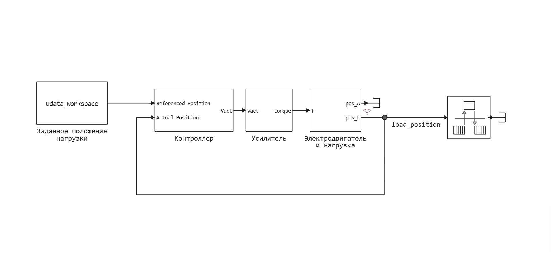
To run a simulation of the model, we need to specify the values of the following parameters:
J1- inertia of the electric motor rotor, ;J2- inertia of the load, ;k- rigidity of the flexible shaft, ;Km- electric motor constant, ;Ka- the gain of the amplifier, ;b1- damping coefficient of electric motor bearings, ;b2- load bearing damping coefficient, ;b12- damping coefficient of the flexible shaft, .
Some of these parameters are known and can be obtained from technical documentation or specialized programs (for example, computer—aided design systems - CAD), including the gain of the amplifier, moments of inertia of the load and the rotor of the electric motor. Other parameters can be determined by direct measurements, such as the stiffness of a flexible shaft. Let's introduce variables containing values of known parameters.:
J1 = 1.00e-6;
J2 = 1.35e-7;
k = 0.001;
Km = 16.4e-3;
Ka = 1.3/2.5;
However, damping coefficients cannot be determined by direct measurements; they must be estimated indirectly based on experimental data on the behavior of the entire system. Therefore, we will set approximate values of these parameters.:
b1 = 1e-5;
b2 = 1e-5;
b12 = 1e-5;
Uploading measurement results
Let's download the values of the measured signals from the "motor_data" experimental data file. In the tdata vector, we will write the values of the time points at which the measurements were carried out, in the udata vector — the input signal representing the specified load position, and in the ydata vector — the output signal corresponding to the measured load position.:
data=read_matfile("$(@__DIR__)/motor_data.mat")
pa_input_voltage = jvector(data["pa_input_voltage"])
pa_output_voltage = jvector(data["pa_output_voltage"])
tdata = jvector(data["tdata"])
udata = jvector(data["udata"])
ydata = jvector(data["ydata"]);
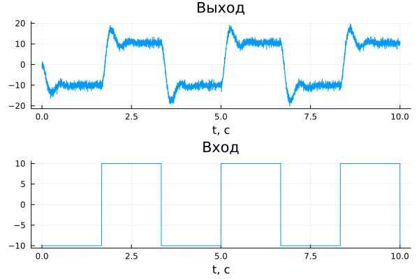
Let's plot the measured signals:
gr()
input = plot(tdata, udata, title = "Entrance", xlabel="t, c",legend=false)
output_measure = plot(tdata, ydata, title = "Exit", xlabel="t, c", legend=false)
plot(output_measure,input,layout = (2, 1))
Comparison of simulation and measurement results
To compare the results of modeling and experimental measurements, it is necessary to provide an input signal to the model and register its output data.
Create a variable of the type WorkspaceArray to transmit the input signal udata into the model. It should be noted that the vector must be used as the time values for the input signal. tdata.
udata_workspace = WorkspaceArray("udata_workspace", DataFrame(time = tdata, value = udata));
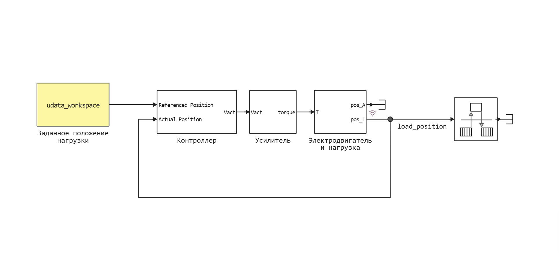
Using the Preset load position block (highlighted in yellow in the image below), the input signal udata_workspace it is transmitted to the input of the controller. The output signal load_position is recorded using logging, and its values become available after the simulation is completed. The Set load position block and the load_position signal correspond to the input and output data collection points of the real system.
Let's open the "motor_pe" model, run its simulation, and then build a graph showing the results of the experiment and simulation.:
model = engee.load("motor_pe.engee")
logout = engee.run(model, verbose=false)
output = plot(tdata, ydata, title = "Exit", xlabel="t, c", label = "experiment", legend=true)
plot!(logout["load_position"].time, logout["load_position"].value, label = "simulation", linewidth=2)
plot(output,input,layout = (2, 1))
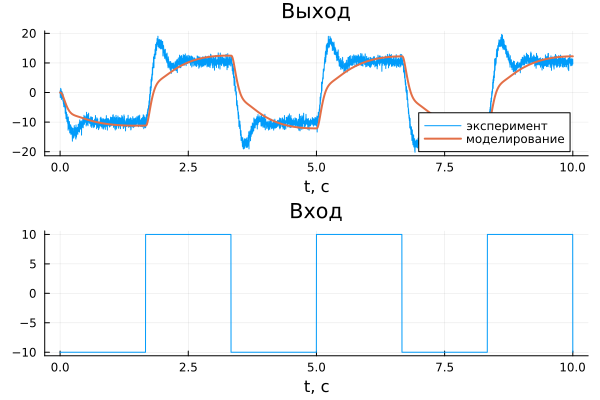
As you can see from the graph, the dynamics of the real system and the model do not match. This indicates the need for more precise adjustment of unknown parameters. b1, b2, b12.
Estimation of parameters using optimization
It is necessary to define such parameter values b1, b2, b21, in which the output signal of the model recorded by the Load position unit corresponds as closely as possible to the measured data ydata.
To do this, we will minimize the sum of the squared errors between the measured and simulated output signals. The errors are calculated as the difference between the values of the measured output signal ydata and the output signal of the load_position model at the time points specified by the vector tdata. To minimize the sum of squared errors, we use one of the available optimization algorithms.
It is important to note that the estimated parameters b1, b2, b21 they must be variables (displayed in the workspace) and used in the model. In this example, they are involved in the motor_pe/Electric Motor and load/State-Space block.
# @markdown # Estimation of model parameters
# @markdown ## To start evaluating the model parameters, enter:
# @markdown ### Model name:
# Opening the model
model_name = "motor_pe" # @param {type:"string"}
if model_name in [m.name for m in engee.get_all_models()] # Checking the condition for loading a model into the kernel
    model = engee.open(model_name) # Open the model
    model = engee.gcm()
else
    @error "Модель $model_name не открыта."
end
# @markdown ### Login (FromWorkspace type block):
input_name = "Заданное положение нагрузки" # @param {type:"string"}
input_path = engee.find_system(model; depth=0, blockparams=["BlockType" => "FromWorkspace","BlockName"=>input_name])
# @markdown ### Input value:
input_data = [tdata udata] # @param {type:"raw"}
typeof(input_data) === Matrix{Float64} || throw(ArgumentError("Входной сигнал должен быть матрицей содержащей числа типа Float64."))
size(input_data,2) == 2 || throw(ArgumentError("Входной сигнал должен иметь 2 столбца - время и значения сигнала."))

isempty(engee.find_system(model; depth=0, blockparams=["BlockType" => "FromWorkspace","BlockName"=>input_name])) && throw(ArgumentError("Блока $input_name не существует в корневой системе модели $(model.name)."))
pe_udata_workspace = WorkspaceArray("pe_udata_workspace", DataFrame(time = input_data[:,1], value = input_data[:,2]));
engee.set_param!("$(model.name)/$input_name", "VariableName" =>"pe_udata_workspace")

# @markdown ### Output (logable signal):
output_name = "load_position" # @param {type:"string"}
output_name in keys(engee.run(model, verbose=false)) || throw(ArgumentError("Сигнал $output_name не найден среди логируемых сигналов."))

# @markdown ### The value of the output signal:
output_data = [tdata ydata] # @param {type:"raw"}
typeof(output_data) === Matrix{Float64} || throw(ArgumentError("Выходной сигнал должен быть матрицей, содержащей числа типа Float64."))
size(output_data,2) == 2 || throw(ArgumentError("Выходной сигнал должен иметь 2 колонки - время и значения сигнала."))

# @markdown ### Names of evaluated parameters:
# Creating a vector of variables, their initial values and constraints
p_names = ["b1","b2","b21"] # @param {type:"raw"}
p_names isa Vector{String} || throw(ArgumentError("Названия параметров должны быть введены в виде вектора строк."))
parametrs_number = length(p_names)
parametrs_number>0 || throw(ArgumentError("Количество параметров должно быть больше нуля."))

# @markdown ### Initial parameter values:
p_0 = [1e-5, 1e-5, 1e-5] # @param {type:"raw"}
p_0 isa Vector{Float64} || throw(ArgumentError("Начальные значения парметров должны быть вектором, содержащим числа типа Float64."))
parametrs_number==length(p_0) || throw(ArgumentError("Количество начальных значений и парметров должно совпадать."))

# @markdown ### Lower bound of parameter values:
p_lower_bounds = [0.0, 0.0, 0.0] # @param {type:"raw"}
p_lower_bounds isa Vector{Float64} || throw(ArgumentError("Нижняя граница значений параметров должна быть вектором, содержащим числа типа Float64."))
parametrs_number==length(p_lower_bounds) || throw(ArgumentError("Количество значений нижней границы и парметров должно совпадать."))

# @markdown ### Upper bound of parameter values:
p_upper_bounds = [1e-3,1e-3,1e-3] # @param {type:"raw"}
p_upper_bounds isa Vector{Float64} || throw(ArgumentError("Верхняя граница значений параметров должна быть вектором, содержащим числа типа Float64."))
parametrs_number==length(p_0) || throw(ArgumentError("Количество начальных значений и парметров должно совпадать."))

# @markdown ## Optimization Settings:
# @markdown ### Optimization algorithm (the "G" at the beginning of the algorithm name indicates that it is global, the "L" is local)
algoritm = :G_MLSL # @param [:GN_DIRECT,:GN_DIRECT_L,:GN_DIRECT_L_RAND,:GN_CRS2_LM,:G_MLSL,:GN_AGS,:GN_ISRES,:GN_ESCH,:LN_COBYLA,:LN_BOBYQA,:LN_PRAXIS,:LN_NELDERMEAD,:LN_SBPLX] {type:"raw"}
# @markdown ### Auxiliary algorithm (only for :G_MLSL)
local_algoritm = :LN_COBYLA # @param [:LN_COBYLA,:LN_BOBYQA,:LN_PRAXIS,:LN_NELDERMEAD,:LN_SBPLX] {type:"raw"}
# Setting optimization parameters
# @markdown ### Minimum relative step change
xtol_rel = 1.0e-1 # @param {type:"number"}
xtol_rel>0 || throw(ArgumentError("Минимальное относительное изменение шага должно быть положительным."))
# @markdown ### Minimum absolute step change
xtol_abs = 1.0e-1 # @param {type:"number"}
xtol_rel>0 || throw(ArgumentError("Минимальное абсолютное изменение шага должно быть больше положительным."))
# @markdown ### Minimal relative change in objective function
ftol_rel = 1.0e-1 # @param {type:"number"}
xtol_rel>0 || throw(ArgumentError("Минимальное относительное изменение целевой функции должно быть положительным."))
# @markdown ### The minimum absolute change in the objective function
ftol_abs = 1.0e-1 # @param {type:"number"}
xtol_rel>0 || throw(ArgumentError("Минимальное абсолютное изменение целевой функции должно быть положительным."))
# @markdown ### Maximum number of estimates of the objective function
maxeval = 30 # @param {type:"integer"}
xtol_rel>0 || throw(ArgumentError("Максимальное количество оценок целевой функции быть больше нуля."))

# @markdown ## Displaying parameter evaluation results
# @markdown ### Graph of measured data and simulation results:
compare = true # @param {type:"boolean"}
# @markdown ### Error graph between measured data and simulation results:
reside = true # @param {type:"boolean"}
# @markdown ### Graph of parameter estimation values:
variables = true # @param {type:"boolean"}
# @markdown ### Graph of objective function values:
objective = true # @param {type:"boolean"}

# Graph comparing the output of the model and the measured data
function compare_plot(model, output_name::String, tdata::Vector{Float64}, udata::Vector{Float64}, ydata::Vector{Float64})
    logout = engee.run(model, verbose=false)
    out_plot = plot(
        logout[output_name].time,
        logout[output_name].value,
        label="simulation",
        title = "Exit",
        xlabel="t, with",
        legend=:bottomright,
        linewidth=3
        )
    plot!(out_plot, tdata, ydata, label="experiment")
    in_plot = plot(tdata, udata, title = "Entrance", xlabel="t, c", legend = false)
    p = plot(out_plot,in_plot,layout = (2, 1), plot_title="Эксперимент и моделирование")
end

# schedule of discrepancies
function residual_plot(model, output_name::String, tdata::Vector{Float64}, ydata::Vector{Float64})
    logout = engee.run(model, verbose=false)
    nearest = interpolate((logout[output_name].time,), logout[output_name].value, Gridded(Constant()))
    residals = ydata .- nearest.(tdata)
    reside = plot(tdata, residals, title = "Mistakes", xlabel="t, with", legend = false)
end

# Schedule of change of variables
function variable_plot(p_names::Vector{String}, parametrs_values)
    p_trace = plot(title = "Parameter values", xlabel="Number of estimates of the objective function",)
    parametrs_values_m = mapreduce(permutedims, vcat, parametrs_values)
    for i in 1:n
        plot!(p_trace, 1:length(parametrs_values_m[:,i]), parametrs_values_m[:,i], markers=:auto, label = p_names[i])
    end
    return p_trace
end

n = parametrs_number

# Vectors for logging the values of the objective function and variables
loss_function_vector = Vector{Float64}()
parametrs_values = Vector{Vector{Float64}}()

# loss function
function myfunc(x::Vector, grad::Vector, output_name::String, measure_time, measure_value, parametrs_name...)
    str = ""
    iterations_value = Vector{Float64}()
    for (value,p) in zip(x, parametrs_name)
        global parametr = Symbol(p)
        @eval(($parametr)=$(value))
        str = str*"$p = $value, "
        push!(iterations_value, value)
    end
    push!(parametrs_values, iterations_value)
    simulation_out = engee.run(model, verbose=false) |> x->collect(x[output_name])
    if measure_time[end]>simulation_out.time[end]
        push!(simulation_out,[measure_time[end], simulation_out.time[end]])
    end
    nearest = interpolate(
        (simulation_out.time,),
        simulation_out.value,
        Gridded(Constant())
    )
    l = sum(abs2, measure_value .- nearest.(measure_time))
    str = "$(length(parametrs_values)). "*str*"loss = $l"
    println(str)
    push!(loss_function_vector, l)
    return l
end


opt = Opt(algoritm, n) # gradient-free algorithm
algoritm === :G_MLSL && NLopt.local_optimizer!(opt, Opt(local_algoritm, n))
opt.lower_bounds = p_lower_bounds
opt.upper_bounds = p_upper_bounds
opt.xtol_rel = xtol_rel
opt.xtol_abs = xtol_abs
opt.ftol_rel = ftol_rel
opt.ftol_abs = ftol_rel
opt.maxeval =  maxeval

opt.min_objective = (x,g) -> myfunc(x,g,output_name,output_data[:,1],output_data[:,2],p_names...)

(minf,minx,ret) = optimize(opt,p_0)
numevals = opt.numevals

str = "\nРезультаты оценки:\n"
for (name, value) in zip(p_names, minx)
    str = str*"$name = $value\n"
end
str = str*"\nЗначение целевой функции = $minf.\n\nОптимизация завершена после $numevals оценок целевой функции cо статусом: $ret.\n"
print(str)

compare && display(compare_plot(model, output_name, input_data[:,1], input_data[:,2], output_data[:,2]))
println("")
reside && display(residual_plot(model, output_name, output_data[:,1], output_data[:,2]))
println("")
objective &&
    display(
        plot(1:numevals, loss_function_vector, title = "Target function", xlabel="Number of estimates of the objective function", legend = false, markers = :circle)
    )
println("")
variables && display(variable_plot(p_names, parametrs_values))
println("")
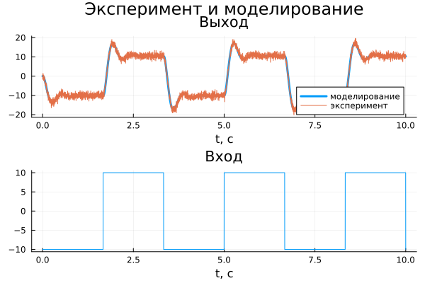


After completing the required number of iterations, the following values of the estimated parameters were obtained:
b1= 2.9731e-6 is the damping coefficient of the electric motor bearings;b2= 9.1799e-23 — load bearing damping coefficient;b12= 7.439e-6 is the damping coefficient of the flexible shaft.
A visual comparison of the simulation and experimental results shows that a fairly accurate match has been achieved between the dynamics of the model and the behavior of the real system. You can also build additional graphs by selecting the appropriate parameters, which will allow for a more detailed analysis of the results.
The quality of parameter estimation depends on the following factors:
- accuracy of the initial parameter values;
- imposed restrictions on parameter values;
- optimization algorithm settings;
- the number of estimated parameters.
Results
In this example, the possibility of estimating unknown parameters included in the equations of the electric drive model based on experimental data is considered. A graph is constructed comparing the results of the simulation and experiment, which demonstrates their coincidence, confirming the correctness of the found parameter values.