Modeling and analysis of asynchronous electric drive operation with scalar control according to the law with feedback on torque and speed.
The example is devoted to modeling and analyzing the operation of an asynchronous electric drive with scalar control according to the law with feedback on torque and speed. Based on the model, Engee demonstrates the possibilities of improving the accuracy of maintaining speed and protecting the drive from overload by introducing negative speed feedback. , positive feedback on the moment (slip compensation) and negative torque feedback (torque limitation at an acceptable level ). The behavior of the rotor speed is considered and the electromagnetic moment during overclocking, steady state, and overloading both with and without feedback loops. The results are relevant for developers of electric drive control systems, where increased speed accuracy and torque overload protection are required without switching to vector control.
Introduction
Scalar asynchronous motor control (AD) is one of the most common methods of speed control in industrial electric drives. Its principle is based on maintaining a preset ratio between the amplitude of the stator voltage and the power supply frequency, which allows you to control the flow in the machine without a rotor position sensor. The method became widespread in the 1970s and 1980s with the advent of affordable voltage inverters based on thyristors and transistors, and today it is implemented in almost all serial frequency converters.
In its basic (open-loop) implementation, scalar control is legally It has a significant disadvantage: the actual speed of the rotor wrwr differs from the set synchronous speed. by the amount of sliding, depending on the moment of loading . When the load changes, the speed "sags", and the system itself is not protected from exceeding the permissible torque. To eliminate these disadvantages without moving to more complex vector control, additional feedbacks are introduced into the structure.:
Negative speed feedback — used in the presence of a speed sensor (DS) and allows you to obtain a more rigid mechanical characteristic of the drive due to the speed controller (RS), which sets the frequency according to misalignment .
Positive torque feedback — used in the absence of a speed sensor and provides slip compensation by evaluating the torque according to the electrical signals of the converter (phase currents and voltages or DC link signals), followed by correction of the output frequency by
Negative torque feedback — implemented by the torque regulator (RM), which limits the engine torque to an acceptable level by reducing the output frequency in case of overload, which protects the drive and the driven mechanism from unacceptable dynamic loads.
The combined use of these feedbacks makes it possible to significantly improve the characteristics of an electric drive with scalar control (to increase the accuracy of maintaining steady-state speed and to limit the torque during loading), while maintaining the relative simplicity of implementation characteristic of scalar control in general.
The example model
Model scalar_control_im_feedback.engee The one considered in this example is recreated by analogy scalar_control_im.slx[1].
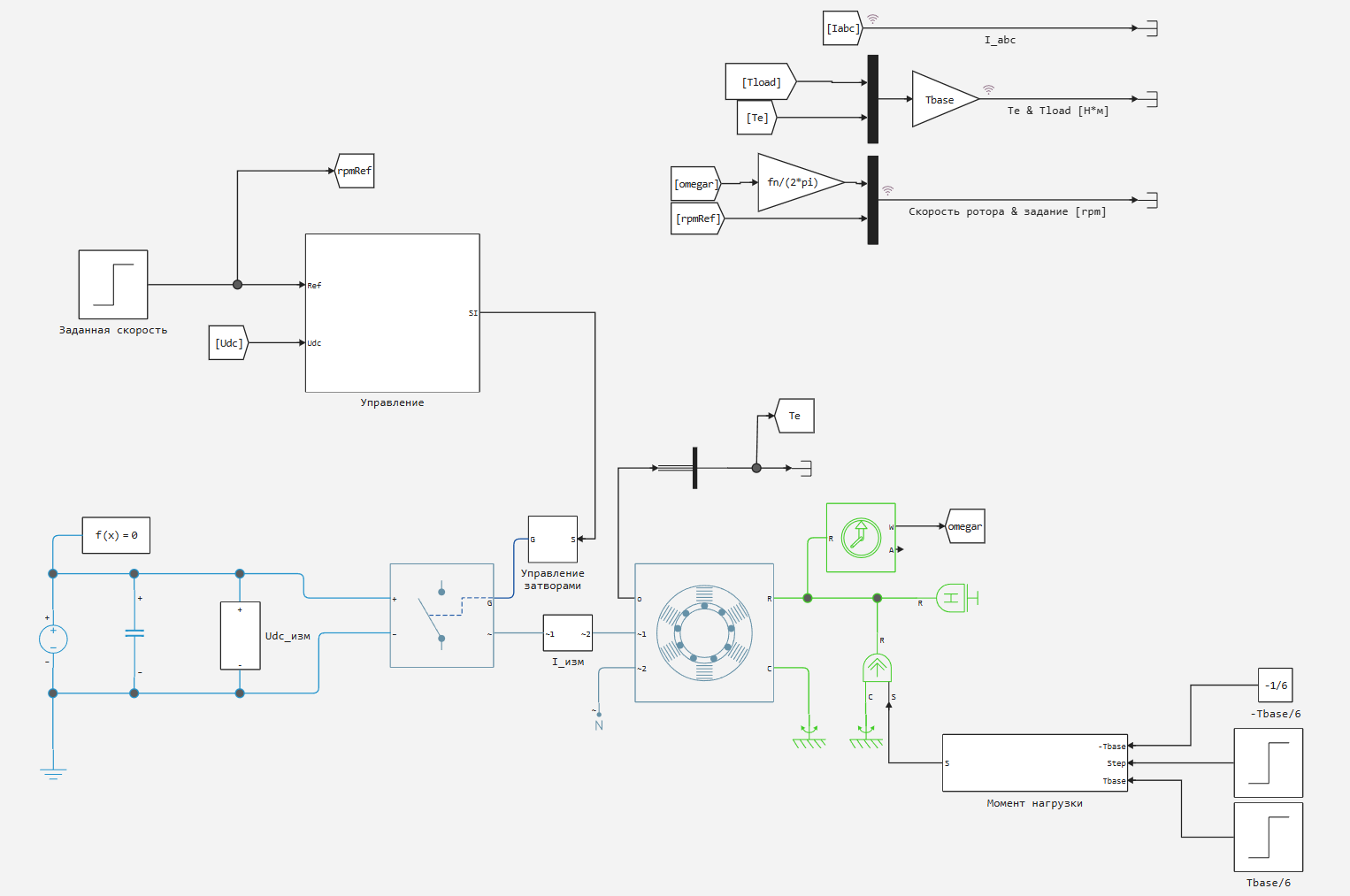
The model consists of a power unit, a control unit, and measurement units. The power unit consists of the following elements:
-
DC link constant voltage source with voltage measurement.
-
A DC link capacitor.
-
Three-phase bridge voltage inverter on ideal semiconductor switches, controlled by gate signals.
-
A three-phase stator current measuring unit with three ammeters, which generates a data array.
-
Asynchronous motor with the replacement circuit parameters shown in Table 1.
-
Rotor angular velocity sensor.
-
A block that generates a stepwise moment of resistance.
Engine parameters are shown in Table 1.
|
Parameter |
Designation |
Value |
|
Rated power |
|
164 kW |
|
Rated voltage (interfacial) |
|
380 V |
|
Rated frequency |
|
50 Hz |
|
Number of pairs of poles |
|
2 |
|
Active resistance of the stator |
|
0.0122 Ohms |
|
Active resistance of the rotor |
|
0.0099 Ohms |
|
Inductive resistance of stator scattering |
|
0.0591 Ohms |
|
Inductive resistance of the rotor scattering |
|
0.0591 Ohms |
|
Stator scattering inductance |
|
0.188 MH |
|
Magnetization resistance |
|
2.39 Ohms |
|
The constant of inertia |
|
0.2734 s |
|
Coefficient of viscous friction |
|
0.0106 O.E. |
The load is generated by the block Момент нагрузки: at the time specified by the signal Step, the moment switches between values and (braking). This reproduces the start, steady state, and load surge/reset.
Description of the operating principle of the control algorithm
The general structure of the "Management" block
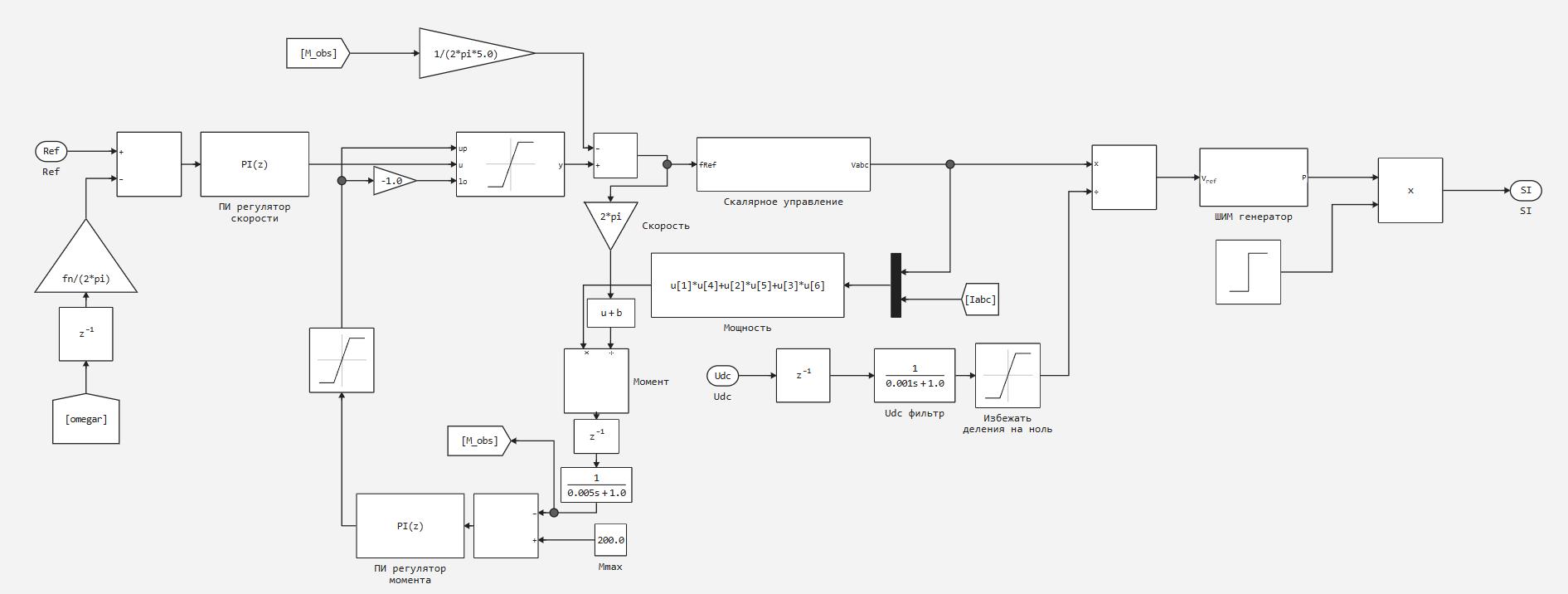
Block Управление accepts the current speed setting as input Ref, the measured voltage of the DC link Udc, phase currents Iabc and the measured speed of the rotor (signal omegar, coming from the engine model). Signal processing implements a structure with speed and torque feedbacks and is performed in the following sequence:
Speed contour. Preset speed Ref it is compared with the speed feedback signal, reduced to rpm by a factor of fn/(2π). The resulting misalignment is sent to the PI speed controller.
Limiting the output frequency and accounting for PM. The output of the PI speed controller is supplied to the input u the block Saturation, the upper and lower limits of which (up, lo) are generated by the signal of the torque regulator (PM) directly as the upper limit and through Gain =-1.0 as the lower one. In this way, negative torque feedback is realized: when the torque exceeds the permissible level, the RM output limits the range of permissible output frequency values from above and below. Saturation result y represents a preset frequency .
Slip compensation. Assessment of the moment (signal M_obs) is passed through an inertial filter and a block Gain ( - preset stiffness), forming a slip compensation additive , which is subtracted from by implementing positive feedback on the moment.
Scalar control. Adjusted frequency fref arrives on the block Скалярное управление, which generates the specified phase voltages Vabc∗ in accordance with the chosen law and compensation regime.
** Assessment of the moment.** Phase currents Iabc and the set phase voltages are multiplied in pairs (block Мощность, u[1]⋅u[4]+u[2]⋅u[5]+u[3]⋅u[6]), forming an estimate of the instantaneous power. After dividing by the current velocity and passing through the inertial filter, a smoothed estimate of the moment is formed. (signal M_obs), used both in the slip compensation circuit and in the torque limitation circuit.
Torque control (RM). Assessment It is compared with the specified allowable moment. , the misalignment is fed to the PI-torque controller, the output of which limits the speed contour, as described above.
Normalization according to Udc. Vector Vabc∗ divided by the filtered value Udc with a limiter to protect against division by zero, converting voltages into relative units of modulation Uref.
PWM generator. Normalized signal Uref it is supplied to a PWM generator with a switching frequency , forming a three-phase set of control signals for the gates of the inverter.
Enabling signal. Step signal Step enables the operation of the PWM generator by multiplying its output signal by 0 or 1.
Block output signal Управление — vector SI, containing six control signals of the inverter gates.
Scalar Control unit
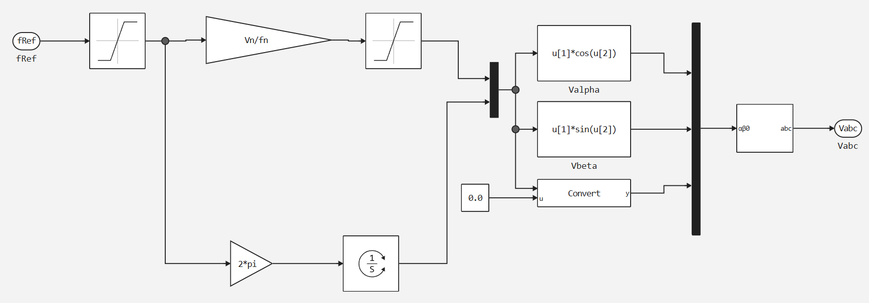
The scalar control unit is the core of the algorithm. A preset frequency is received at its input .
Based on A preset voltage is generated:
Formation of three-phase voltages
From a given frequency The voltage angle is calculated by integration:
Set voltage and the angle They are used to construct a three-phase voltage vector in a coordinate system. :
Then the vector (, , ) is converted from the coordinate system into a three-phase coordinate system by block Преобразование αβ0 в abc:
The resulting vector it goes to the output of the scalar control unit and then to the normalization and PWM generator.
The Shutter Control unit
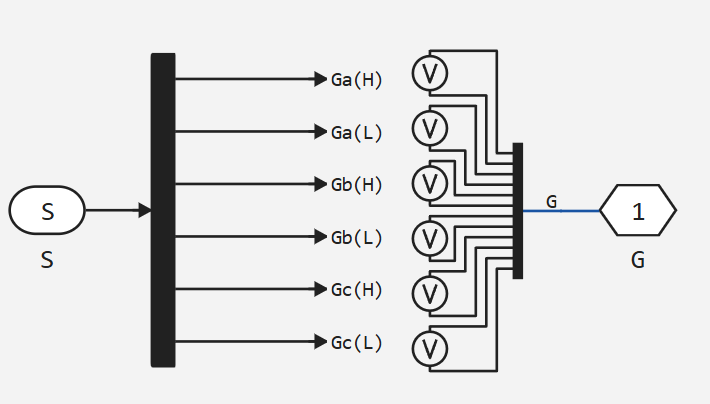
Block Управление затворами receives a vector of signals S and generates six control signals of the inverter gates: Ga(H), Ga(L), Gb(H), Gb(L), Gc(H), Gc(L) — a pair for each shoulder of the bridge (upper and lower keys). The signals of the upper and lower keys of the same arm are complementary, taking into account dead time. Output signal G it is transmitted to the power circuit of the inverter.
The "Load moment" block
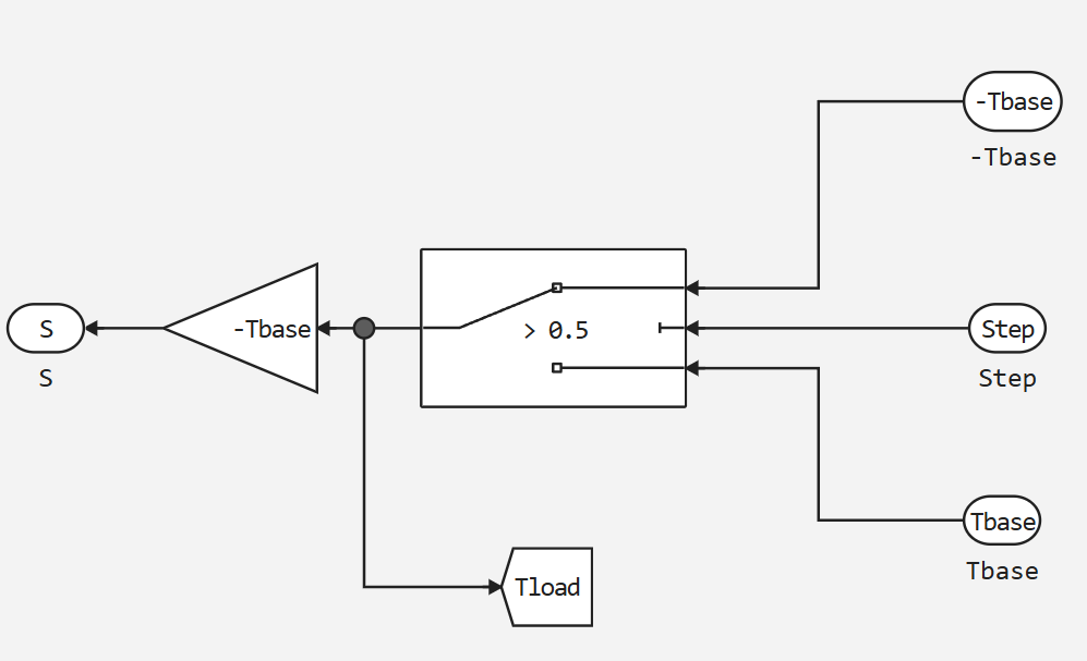
The block generates the load moment acting on the motor shaft. The switch selects between the values and depending on the signal Step (switching threshold 0.5). The output torque is scaled by the coefficient −Tbase (the minus sign is the load torque directed against rotation). The signal at the same time, it is displayed in the model space for display on the graph.
Simulation
The simulation is performed under the following scenario:
-
At the moment t = 0.4, the speed is set = 800 rpm.
-
When the set speed is reached, the engine operates in steady state without load.
-
At a given time (
Step) The rated load torque is applied , after which the load is reset or the sign changes.
Simulation Parameters:
|
Parameter |
Value |
|
Basic sampling step |
5 microseconds |
|
Switching frequency |
2 kHz |
|
Set speed |
800 rpm |
The next code cell will start the simulation:
model_name = "induction_motor_scalar_feedback"
model_path = "$(@__DIR__)/$model_name.engee"
engee.load(model_path) |> engee.run; # uploaded and executed the model
engee.close(engee.gcm(), force=true) # the model was closed
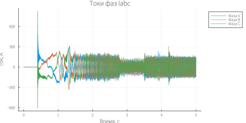
Next, we will plot the instantaneous phase currents.:
gr(size=(800, 400))
p = WorkspaceArrays.plot_wa(WorkspaceArray{Vector{Float64}}("$model_name/I_abc"))
xlabel!(p, "Time, from")
ylabel!(p, "Current, A")
title!(p, "Iabc Phase Currents")

p[1][1][:label] = "Фаза A"
p[1][2][:label] = "Фаза B"
p[1][3][:label] = "Фаза C"

plot!(p, legend=:outertopright)
# p
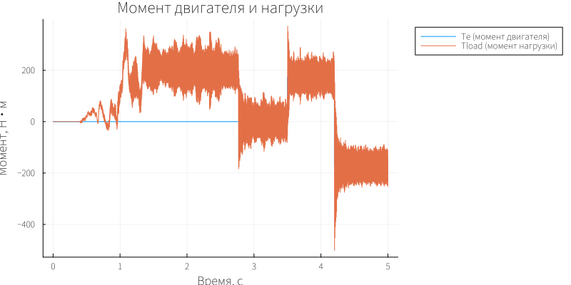
Graphs of load moment and engine moment:
p = WorkspaceArrays.plot_wa(WorkspaceArray{Vector{Float64}}("$model_name/Te & Tload [Н*м]"))
xlabel!(p, "Time, from")
ylabel!(p, "The moment, N·m")
title!(p, "Motor and load torque")

p[1][1][:label] = "Te (момент двигателя)"
p[1][2][:label] = "Tload (момент нагрузки)"

plot!(p, legend=:outertopright)
# p
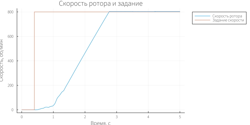
Graphs of the set and actual angular velocity:
p = WorkspaceArrays.plot_wa(WorkspaceArray{Vector{Float64}}("$model_name/Скорость ротора & задание [rpm]"))
xlabel!(p, "Time, from")
ylabel!(p, "Скорость, об/мин")
title!(p, "Rotor speed and setting")

p[1][1][:label] = "Скорость ротора"
p[1][2][:label] = "Задание скорости"

plot!(p, legend=:outertopright)
# p
During acceleration, the electromagnetic torque of the engine (orange curve) reaches values of the order of 200 Nm (the maximum torque that was set in the control system), after which it decreases to zero as it reaches steady speed. In the range t≈2.7–3.5 s, the engine is idling — the torque is close to zero. At the moment t ≈ 3.5 s, a load moment is applied = (blue curve): Te takes a value of about 180 Nm. At t ≈ 4.2 s, the load changes sign to , the electromagnetic moment becomes negative -180 Nm . Throughout the simulation, ripples of a moment with a switching frequency characteristic of a PWM inverter are observed.
The stator currents (phases a, b, and c — blue, orange, and yellow curves) reach an amplitude of about 800 A during acceleration, which corresponds to the starting mode. In steady-state idle mode, the amplitude decreases to ≈100 A. After loading at t ≈ 3.5 s, the currents increase to 180 A with characteristic PWM ripples. When the load sign changes in t≈4.2 s, the amplitude of the currents decreases to 140 A.
Rotor speed (orange curve) follows the assignment rpmRef (blue curve): The speed is set at the target level of 800 rpm. When the load is applied, there is no static velocity error, which is due to the sliding compensation by the regulator.
Conclusion
The example simulates the operation of an asynchronous electric drive with scalar control according to the law with feedback on torque and speed in the Engee environment, which confirmed the operability of the proposed control structure during acceleration, steady state and load surge. It is shown that the introduction of negative feedback on speed allows you to eliminate the static error characteristic of open scalar control, the actual speed of the rotor in steady state exactly matches the target, and does not lag behind it by the amount of slip. The torque regulator (RM) implemented in the model ensures the limitation of the electromagnetic moment engine capacity of 164 kW at an acceptable level when setting and changing the load sign, thereby protecting the drive and the driven mechanism from unacceptable dynamic overloads. The simulation results confirm that scalar speed and torque feedback control provides significantly higher accuracy of speed maintenance and torque protection compared to an open-loop system, approaching the static characteristics of subordinate control systems, while maintaining the relative simplicity of implementation characteristic of scalar control. The model can serve as a basis for further investigation of the influence of speed and torque control parameters (PI control coefficients, the time constant of the torque estimation filter) on the quality of regulation, as well as a starting point for the transition to more complex algorithms - vector and direct torque control.
Used sources
- Asynchronous Machine Scalar Control — MathWorks Documentation
- Anuchin A. S. Control systems of electric drives : textbook for universities. Moscow : MEI Publishing House, 2015. 371 p. ISBN 978-5-383-00918-5.