Evaluation of the parameters of the electric drive model
Modeling often involves a situation where the laws describing the behavior of an object are known, but some parameters included in the equations remain uncertain. In this example, the process of estimating unknown parameters of an electric drive model based on experimental data is considered in stages.
Connecting the necessary packages
Install the necessary packages:
import Pkg
Pkg.add(["Interpolations","NLopt"])
We will connect the necessary packages:
using DataFrames, Plots,Interpolations, NLopt, MATLAB
Electric drive model
Consider the "motor_pe" electric drive model, the diagram of which is shown in the figure below. It consists of a controller, an amplifier and an electric motor with a load. The input of the model is a signal controlling the load position, the output is the load position.
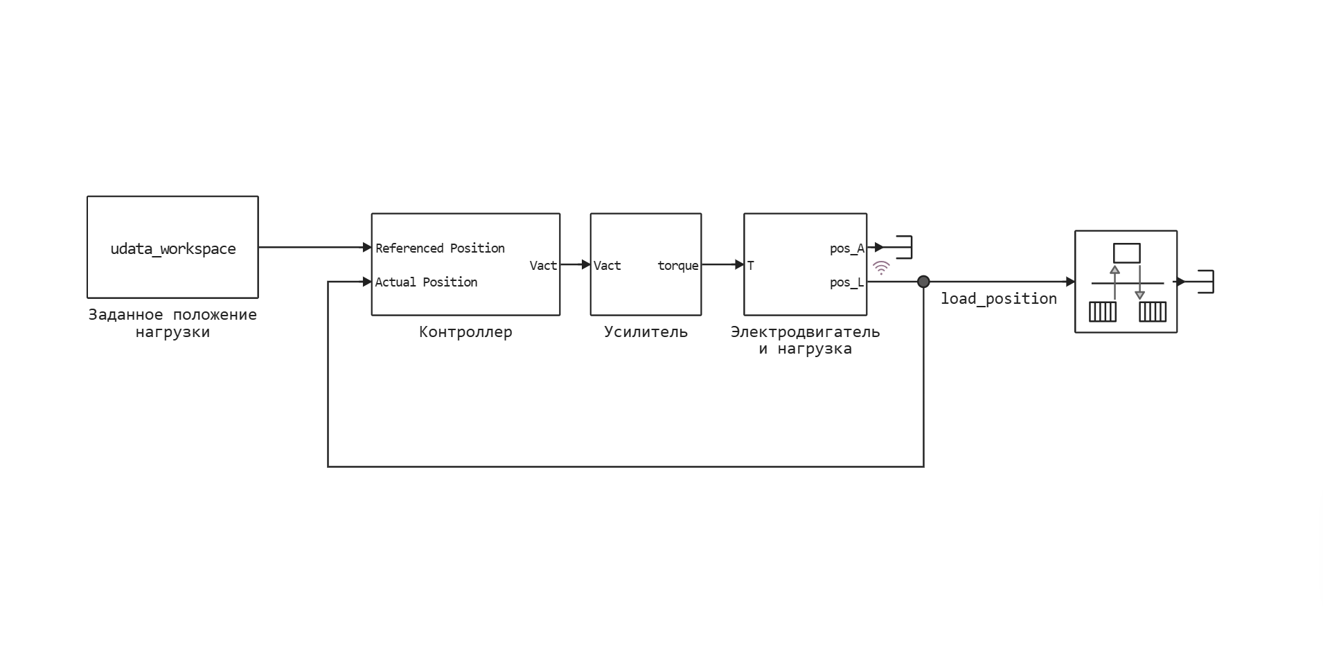
To run a simulation of the model, we need to specify the values of the following parameters:
J1- inertia of the electric motor rotor, ;J2- inertia of the load, ;k- rigidity of the flexible shaft, ;Km- electric motor constant, ;Ka- the gain of the amplifier, ;b1- damping coefficient of electric motor bearings, ;b2- load bearing damping coefficient, ;b12- damping coefficient of the flexible shaft, .
Some of these parameters are known and can be obtained from technical documentation or specialized programs (for example, computer—aided design systems - CAD), including the gain of the amplifier, moments of inertia of the load and the rotor of the electric motor. Other parameters can be determined by direct measurements, such as the stiffness of a flexible shaft. Let's introduce variables containing values of known parameters.:
J1 = 1.00e-6;
J2 = 1.35e-7;
k = 0.001;
Km = 16.4e-3;
Ka = 1.3/2.5;
However, damping coefficients cannot be determined by direct measurements; they must be estimated indirectly based on experimental data on the behavior of the entire system. Therefore, we will set approximate values of these parameters.:
b1 = 1e-5;
b2 = 1e-5;
b12 = 1e-5;
Uploading measurement results
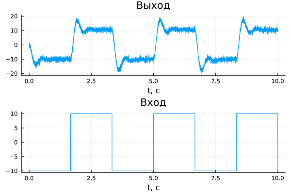
Let's download the values of the measured signals from the "motor_data" experimental data file. In the tdata vector, we will write the values of the time points at which the measurements were carried out, in the udata vector — the input signal representing the specified load position, and in the ydata vector — the output signal corresponding to the measured load position.:
data=read_matfile("$(@__DIR__)/motor_data.mat")
pa_input_voltage = jvector(data["pa_input_voltage"])
pa_output_voltage = jvector(data["pa_output_voltage"])
tdata = jvector(data["tdata"])
udata = jvector(data["udata"])
ydata = jvector(data["ydata"]);
Let's plot the measured signals:
gr()
input = plot(tdata, udata, title = "Entrance", xlabel="t, c",legend=false)
output_measure = plot(tdata, ydata, title = "Exit", xlabel="t, c", legend=false)
plot(output_measure,input,layout = (2, 1))
Comparison of simulation and measurement results
To compare the results of modeling and experimental measurements, it is necessary to provide an input signal to the model and register its output data.
Create a variable of the type WorkspaceArray to transmit the input signal udata into the model. It should be noted that the vector must be used as the time values for the input signal. tdata.
udata_workspace = WorkspaceArray("udata_workspace", DataFrame(time = tdata, value = udata));
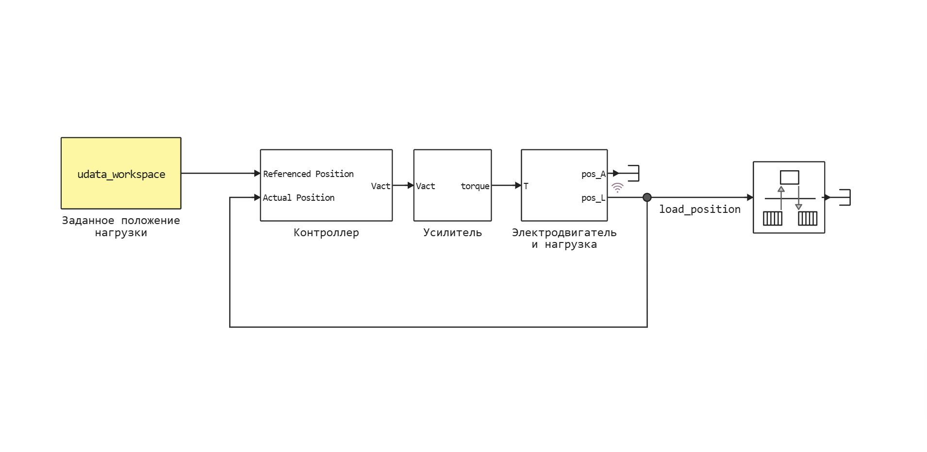
Using the Preset load position block (highlighted in yellow in the image below), the input signal udata_workspace it is transmitted to the input of the controller. The output signal load_position is recorded using logging, and its values become available after the simulation is completed. The Set load position block and the load_position signal correspond to the input and output data collection points of the real system.
Let's open the "motor_pe" model, run its simulation, and then build a graph showing the results of the experiment and simulation.:
model = engee.load("motor_pe.engee")
logout = engee.run(model, verbose=false)
output = plot(tdata, ydata, title = "Exit", xlabel="t, c", label = "experiment", legend=true)
plot!(logout["load_position"].time, logout["load_position"].value, label = "simulation", linewidth=2)
plot(output,input,layout = (2, 1))
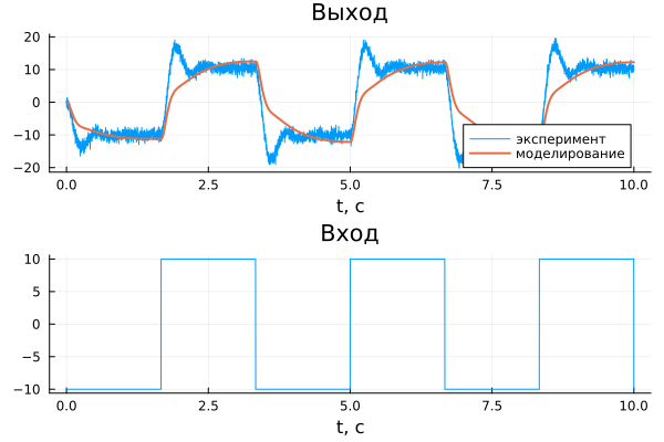
As you can see from the graph, the dynamics of the real system and the model do not match. This indicates the need for more precise adjustment of unknown parameters. b1, b2, b12.
Estimation of parameters using optimization
It is necessary to define such parameter values b1, b2, b21, in which the output signal of the model recorded by the Load position unit corresponds as closely as possible to the measured data ydata.
To do this, we will minimize the sum of the squared errors between the measured and simulated output signals. The errors are calculated as the difference between the values of the measured output signal ydata and the output signal of the load_position model at the time points specified by the vector tdata. To minimize the sum of squared errors, we use one of the available optimization algorithms.
It is important to note that the estimated parameters b1, b2, b21 they must be variables (displayed in the workspace) and used in the model. In this example, they are involved in the motor_pe/Electric Motor and load/State-Space block.
Masks only work in the Code Editor, so here is a screenshot of the interface that will be available to you after opening the motor_pe.ngscript file.

After completing the required number of iterations, the following values of the estimated parameters were obtained:
b1= 2.9731e-6 is the damping coefficient of the electric motor bearings;b2= 9.1799e-23 — load bearing damping coefficient;b12= 7.439e-6 is the damping coefficient of the flexible shaft.
A visual comparison of the simulation and experimental results shows that a fairly accurate match has been achieved between the dynamics of the model and the behavior of the real system. You can also build additional graphs by selecting the appropriate parameters, which will allow for a more detailed analysis of the results.
The quality of parameter estimation depends on the following factors:
- accuracy of the initial parameter values;
- imposed restrictions on parameter values;
- optimization algorithm settings;
- the number of estimated parameters.
Results
In this example, the possibility of estimating unknown parameters included in the equations of the electric drive model based on experimental data is considered. A graph is constructed comparing the results of the simulation and experiment, which demonstrates their coincidence, confirming the correctness of the found parameter values.