Trapezoidal (six-step) BDPT control (BLCD)
This project shows a trapezoidal (six-step) control model BDPT (BLDC).
Introduction
Trapezoidal BDT control is a system without feedback on speed or current.
Hall sensors that determine the position of the motor shaft are used only for switching motor windings. The figure below shows a block diagram of such a management model.
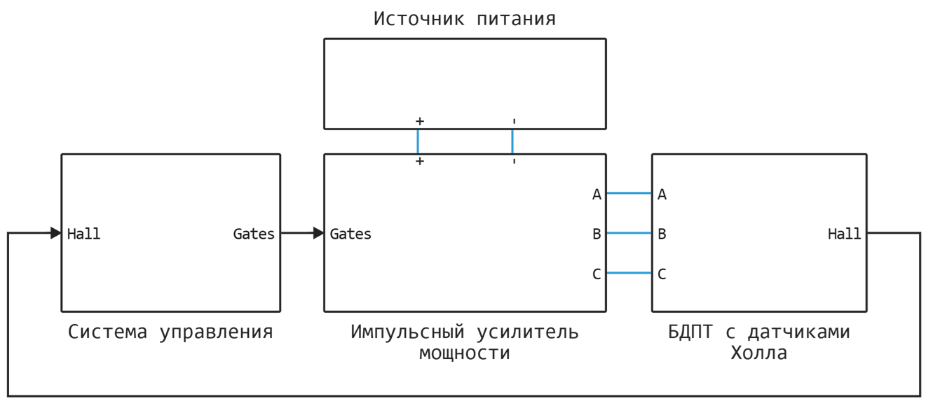
The model consists of the following elements:
- Control system (SU);
- Switching power amplifier (IUM);
- Power supply (IP);
- BDPT with Hall sensors.
Key Elements (CE) IUM are selected based on field effect transistors (MOSFETs).
The model implements the possibility of choosing the switching method and the control method of the KE IUM, as well as the connection scheme of the BDPT phases.
For more information about the electric motor control system, on which the model developed here is based, see [1].
The management system
The SU developed for this example is based on truth tables (each for its own control method), and they, in turn, define the control function of the QE and the IUM.
The device of the BDPT SU is shown below.
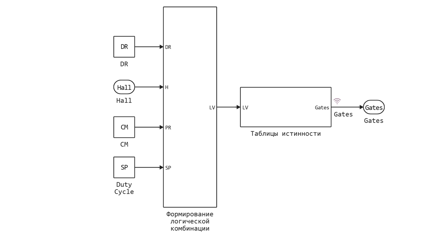
The control function of the QE IUM is formed using a logical combination of 4 variables:
DR- the direction of rotation of the engine (0- direct rotation,1- the opposite);H- position signals from Hall sensors;PR- defines the switching method of the KU IUM (PWM fill factor);SP- sets the speed (PWM fill factor).
KE and KUM switching methods
The switching method of CE and IUM affects the load distribution between CE and is determined using a constant CM. Three switching methods are used:
- Non-symmetrical (bottom)
CD = 0; - Unbalanced (upper)
CD = 100; - Alternate
CD = 50.
When CM = 0, which means that PR = 0, the lower CES are loaded more than the upper ones.
In the case when CM = 100, PR = 1, then, on the contrary, the lower CES are loaded more.
If CM = 50 and, accordingly, PR = 0,5, the upper and lower CES are equally loaded during the PWM period.
The method of managing CE and IUM
There are 3 ways to control the control panel: 120-degree, 150-degree and 180-degree.
The control method is determined by the number of installed Hall sensors and their relative position.
In 120- and 180-degree control methods, it is necessary to divide the position of the motor shaft into 6 sectors, for which you need to install 3 Hall sensors.
The 150-degree switching allows for the use of 6 Hall sensors, which means a division into 12 sectors.
For example, the location of the sensors used in the engine model is shown below, in which the phases are connected according to the "star" scheme (wye) with various methods of managing CE and IUM.
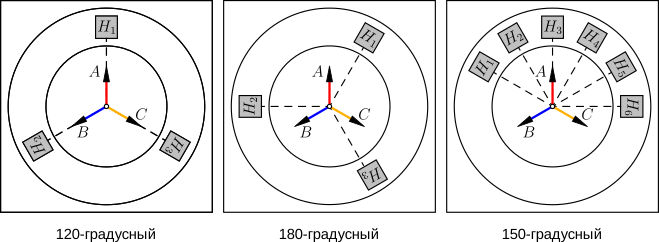
For the "triangle" connection diagram (Delta) all Hall sensors are rotated to radians clockwise.
The algorithm for determining the position using Hall sensors is based on their displacement relative to each other.
The offset is shown below bias Hall sensors H when connecting the phases of the engine according to the "star" scheme and various control methods of the KE IUM.
[PIPE] H [PIPE] bias (120)[PIPE] bias (180)[PIPE] bias (150)[PIPE]
[PIPE] ---------- [PIPE]:---------:[PIPE]:---------:[PIPE]:---------:[PIPE]
[PIPE] H1 [PIPE] [PIPE] [PIPE] [PIPE]
[PIPE] H2 [PIPE] [PIPE] [PIPE] [PIPE]
[PIPE] H3 [PIPE] [PIPE] [PIPE] [PIPE]
[PIPE] H4 [PIPE] [PIPE] [PIPE] [PIPE]
[PIPE] H5 [PIPE] [PIPE] [PIPE] [PIPE]
[PIPE] H6 [PIPE] [PIPE] [PIPE] [PIPE]
Simulation
We will connect the necessary expansion packs:
# Connecting the necessary packages
using CSV
Using a macro @__DIR__ define the descriptor of the path to the project files:
demoroot = @__DIR__;
Data and parameters
Download the data from the truth tables:
# Downloading truth tables from a CSV file
truthTable120d = CSV.read("$demoroot/data/truthTable120d.csv",
                         DataFrame; delim = ",", header = false);
truthTable150d = CSV.read("$demoroot/data/truthTable150d.csv",
                         DataFrame; delim = ",", header = false);
truthTable180d = CSV.read("$demoroot/data/truthTable180d.csv",
                         DataFrame; delim = ",", header = false);

# Ways to manage QE IUM
# # 120-degree
tt120deg = truthTable120d.Column1;
tt120deg = [tt120deg truthTable120d.Column2];
tt120deg = [tt120deg truthTable120d.Column3];
tt120deg = [tt120deg truthTable120d.Column4];
tt120deg = [tt120deg truthTable120d.Column5];
tt120deg = [tt120deg truthTable120d.Column6];

# # 150-degree
tt150deg = truthTable150d.Column1;
tt150deg = [tt150deg truthTable150d.Column2];
tt150deg = [tt150deg truthTable150d.Column3];
tt150deg = [tt150deg truthTable150d.Column4];
tt150deg = [tt150deg truthTable150d.Column5];
tt150deg = [tt150deg truthTable150d.Column6];

# # 180-degree
tt180deg = truthTable180d.Column1;
tt180deg = [tt180deg truthTable180d.Column2];
tt180deg = [tt180deg truthTable180d.Column3];
tt180deg = [tt180deg truthTable180d.Column4];
tt180deg = [tt180deg truthTable180d.Column5];
tt180deg = [tt180deg truthTable180d.Column6];
We will set the parameters of modeling, IP, BDPT and IUM:
# Simulation Parameters
Ts = 5e-6; # Sampling time of the physical mode

# IP parameters
Us = 24; # Supply voltage, V

# BDPT Parameters
R  = 2.25;             # Resistance of the stator winding, ohms
L  = 0.0032;           # Inductance of the stator winding, Gn
Cm = 0.03397;          # The moment constant, N*m/A
Ce = 0.0258;           # Permanent anti-EMF, V*s/rad
J  = 2.4e-6;           # Moment of inertia of the rotor, kg*m^2
Bm = 0;                # Rotor damping, N*m*s/rad
p  = 4;                # Number of pairs of poles
Fmax = (2/3)*(Cm/p);   # The maximum value of the flux coupling of permanent magnets
ThetaConst = pi/(2*p); # The angle of the rotor at which the EMF is constant

# IUM Parameters
f     = 5000;  # Switching frequency, Hz
Rds   = 4e-2;  # Drain-source resistance, Ohms
Goffs = 1e-6;  # Conductivity in the switched-off state, Cm
Uthr  = 0.5;   # Threshold voltage, V
Udf   = 0.8;   # The forward voltage of the integrated diodes, In
Ron   = 1e-3;  # Resistance of integrated diodes when switched on directly, Ohms
Goff  = 1e-5;  # Conductivity of integrated diodes in the closed state, See
Csn   = 1e-7;  # Snubber capacity, F
Rsn   = 1e4;   # Snubber resistance, Ohms
The choice of the switching method of the KE IUM is carried out by defining a variable comType the corresponding number (120/150/180).
# Choosing the switching method of CE and IUM
comType = 120; # 120 / 150 / 180
Similarly, using a variable woundType The connection scheme of the engine phases is selected. Here, the "triangle" type scheme corresponds to 1, and the type of "star" - 2.
# # Selection of the motor phase connection scheme
woundType = 1; # triangle = 1, star = 2

# Loading the Engee model if it is not already open on the canvas
if "bldc_control_sixstep" ∉ getfield.(engee.get_all_models(), :name)
    engee.load( "$demoroot/bldc_control_sixstep.engee");
end

bldc_root = "bldc_control_sixstep/БДПТ с датчиками Холла/БДПТ";
if woundType == 1
    engee.set_param!(bldc_root, "winding_type" => "Delta-wound")
elseif woundType == 2
    engee.set_param!(bldc_root, "winding_type" => "Wye-wound")
    engee.set_param!(bldc_root, "zero_sequence" => "Exclude")
end
Finally, we define the variables of the switching method CE and IUM CM, directions DR and speed SP rotation of the motor shaft:
CM = 0;   # 0 - unbalanced (lower) 100 - unbalanced (upper), 50 - alternating
DR = 0;   # 0 - forward rotation, 1 - reverse
SP = 100; # PWM [0...100] - % of the maximum engine speed
Open the model and run the simulation.:
# Running a simulation of the Engee model
model_data = engee.run("bldc_control_sixstep");
Let's extract the data that was obtained during the simulation.:
angle = model_data["Angle"].value[1:10:end];  # Angle of rotation of the motor shaft, deg
speed = model_data["Speed"].value[1:10:end];  # Engine shaft rotation speed, rpm

# Currents
is = model_data["is"].value[1:10:end];  # Consumption current from the IP
ia = model_data["ia"].value[1:10:end];  # Current of phase A
ib = model_data["ib"].value[1:10:end];  # Current of phase B
ic = model_data["ic"].value[1:10:end];  # Current of phase C

# Voltage
Ua = model_data["Ua"].value[1:10:end];   # Phase voltage A
Ub = model_data["Ub"].value[1:10:end];   # Phase voltage B
Uc = model_data["Uc"].value[1:10:end];   # Phase voltage C
Uab = model_data["Uab"].value[1:10:end]; # Line voltage C
Ubc = model_data["Ubc"].value[1:10:end]; # Line voltage C
Uca = model_data["Uca"].value[1:10:end]; # Line voltage C

# Hall Sensors H
Hall = model_data["Hall"].value[1:10:end];

Hall_1 = zeros(Float64, length(Hall));
Hall_2 = zeros(Float64, length(Hall));
Hall_3 = zeros(Float64, length(Hall));

for i = 1:length(Hall)
    Hall_1[i] = Hall[i][1];
    Hall_2[i] = Hall[i][2];
    Hall_3[i] = Hall[i][3];
end

if comType == 150
    Hall_4 = zeros(Float64, length(Hall));
    Hall_5 = zeros(Float64, length(Hall));
    Hall_6 = zeros(Float64, length(Hall));

    for i = 1:length(Hall)
        Hall_4[i] = Hall[i][4];
        Hall_5[i] = Hall[i][5];
        Hall_6[i] = Hall[i][6];
    end
end

# Key elements of G
Gates = model_data["Gates"].value[1:10:end];

Gates_1 = zeros(Float64, length(Gates));
Gates_2 = zeros(Float64, length(Gates));
Gates_3 = zeros(Float64, length(Gates));
Gates_4 = zeros(Float64, length(Gates));
Gates_5 = zeros(Float64, length(Gates));
Gates_6 = zeros(Float64, length(Gates));

for i = 1:length(Gates)
    Gates_1[i] = Gates[i][1];
    Gates_2[i] = Gates[i][2];
    Gates_3[i] = Gates[i][3];
    Gates_4[i] = Gates[i][4];
    Gates_5[i] = Gates[i][5];
    Gates_6[i] = Gates[i][6];
end
Results
Let's plot the position and speed of the BDPT rotor.:
# gr()      # Disabling interactivity when plotting graphs (easier to draw)
plotlyjs() # Enabling interactivity (harder to draw)
t = model_data["Angle"].time[1:10:end]; # Simulation time, s
plot(
    plot(t, angle, ylabel = "Angle of rotation, degree", lw = 1.5, c = "red",
    title = ""),
    plot(t, speed, xlabel = "Time, from", lw = 1.5, c = "green",
    ylabel = "Скорость, об/мин"),
    layout = (2,1), legend=:false, link=:x
)
Graphs of phase currents and power supply current:
# gr()      # Disabling interactivity when plotting graphs (easier to draw)
plotlyjs() # Enabling interactivity (harder to draw)
t = model_data["is"].time[1:10:end]; # Simulation time, s
plot(
    plot(t, is, ylabel = "Power supply, And", lw = 1.5, c = "black",
    title = "Currents"),
    plot(t, [ia, ib, ic], lw = 1.5, c = ["red" "blue" "yellow"],
    xlabel = "Time, from", ylabel = "Phase-based, And"),
    layout = (2,1), legend=:topright, label = ["is" "ia" "ib" "ic"], link=:x
)
Below are graphs of motor voltages, signals from Hall sensors and on the control panel.
# gr()      # Disabling interactivity when plotting graphs (easier to draw)
plotlyjs() # Enabling interactivity (harder to draw)
t = model_data["Ua"].time[1:10:end]; # Simulation time, s
plot(
    plot(t, [Ua, Ub, Uc], ylabel = "Phase, In", lw = 1.5, c = ["red" "blue" "yellow"],
    title = "BDPT Voltage", label = ["Ua" "Ub" "Uc"]),
    plot(t, [Uab, Ubc, Uca], lw = 1.5, c = ["red" "blue" "yellow"],
    xlabel = "Time, from", ylabel = "Linear, In", label = ["Uab" "Ubc" "Uca"]),
    layout = (2,1), legend=:right, link=:x
)
# gr()      # Disabling interactivity when plotting graphs (easier to draw)
plotlyjs() # Enabling interactivity (harder to draw)
t = model_data["Hall"].time[1:10:end]; # Simulation time, s
if comType == 150
plot(
    plot(t, Hall_1, ylabel = "H1", lw = 1.5,
    title = "Signals from Hall sensors"),
    plot(t, Hall_2, lw = 1.5,
    ylabel = "H2"),
    plot(t, Hall_3, lw = 1.5,
    ylabel = "H3"),
    plot(t, Hall_4, lw = 1.5,
    ylabel = "H4"),
    plot(t, Hall_5, lw = 1.5,
    ylabel = "H5"),
    plot(t, Hall_6, lw = 1.5,
    ylabel = "H6", xlabel = "Time, from"),
    layout = (6,1), legend=:none, link=:x
)
else
    plot(
        plot(t, Hall_1, ylabel = "H1", lw = 1.5,
        title = "Signals from Hall sensors"),
        plot(t, Hall_2, lw = 1.5,
        ylabel = "H2"),
        plot(t, Hall_3, lw = 1.5,
        ylabel = "H3", xlabel = "Time, from"),
        layout = (3,1), legend=:none, link=:x
    )
end
# gr()      # Disabling interactivity when plotting graphs (easier to draw)
plotlyjs() # Enabling interactivity (harder to draw)
t = model_data["Gates"].time[1:10:end]; # Simulation time, s
plot(
    plot(t, Gates_1, ylabel = "G1", lw = 1.5,
    title = "Signals on the KE IUM"),
    plot(t, Gates_2, lw = 1.5,
    ylabel = "G2"),
    plot(t, Gates_3, lw = 1.5,
    ylabel = "G3"),
    plot(t, Gates_4, lw = 1.5,
    ylabel = "G4"),
    plot(t, Gates_5, lw = 1.5,
    ylabel = "G5"),
    plot(t, Gates_6, lw = 1.5,
    ylabel = "G6", xlabel = "Time, from"),
    layout = (6,1), legend=:none, link=:x
)
Conclusion
This project shows a 6-step BDT switching model (BLDC).
The structure, principle of operation and execution options of this type of control are considered.
As a result of the simulation, diagrams of currents, voltages, and logic signals from Hall sensors and on key elements of a DC converter were obtained.
The developed model can be used, for example, as an actuating element of an electric drive.
List of sources used
- Krivilev A.V. Development and implementation on FPGAs of energy—efficient methods of pulse control of "power amplifier - electric motor" systems based on computer-aided
design methods: abstract of the dissertation of the Doctor of Technical Sciences.Sciences, Moscow : MAI, 2013.