A soft-start device for an engine with a fan load
Introduction
A soft starter device (abbreviated as softstarter) is used for controlled start-up and, where required, shutdown of an asynchronous motor. Typical units are fans, pumps, compressors, conveyors, crushers and mills. The SCP gradually increases the motor voltage, reducing inrush current and mechanical shocks in the transmission and load. For a fan with high inertia, this helps reduce the load on belts, bearings, and the network during acceleration.
The advantages of the SCP are setting the time and initial start–up voltage, reducing network drawdowns and mechanical stresses, and after bypass bypass, lower losses in the power part. Limitations – when the voltage is lowered, the available torque also decreases; a heavy load may not be able to accelerate. The SCP does not provide long-term speed control, and thyristor control creates harmonics during start-up. The settings and thermal stability should be checked for a specific unit and the frequency of starts [1].
The example implements the calculation and verification of the model softstarter.engee: acceleration of an asynchronous motor with a mechanical rated power of 15 kW from a three-phase thyristor UPR, then shunting the thyristors with a bypass contactor.
The theoretical part
In each phase of the SCP, a pair of counter-parallel thyristors changes the operating voltage of the motor by means of the release angle . At the start, a large angle limits the voltage; reducing increases it. All other things being equal, the starting electromagnetic moment is approximately proportional to the square of the voltage. This approximation is useful for tuning, but it does not replace the calculation of the transient process with harmonics and inertia[1]. Dependences (1) explain why, when the voltage is lowered, it is necessary to check the sufficiency of the starting torque.
After overclocking, the thyristors are almost completely open. A contactor connected in parallel with the SCP accepts the load current and reduces losses in the power regulator. To evaluate switching, the same time windows before and after the short circuit, the local current maximum and the speed are compared [1, 5].
Initial data and calculation of parameters
For the reproduced example, the AIR160S2 engine is accepted according to the catalog [2]. The rated power of 15 kW is mechanical power . The rated total electrical power for the machine unit is calculated separately. The inertia of the fan without a load passport is an assumption. The initial data is summarized in table 1.
The total power and rated torque are determined by formulas (2) and (3).
Table 1 - Passport data and assumptions
| Value | Meaning | Footing |
|---|---|---|
| 15 kW | engine passport [2] | |
| , | 380 V, 50 Hz | passport [2] |
| , | 2930 rpm, 1 pair of poles | passport [2] |
| , | 0.894; 0.89 | passport [2] |
| , | 28.6 A; 7.5 | passport [2] |
| , | 2.2; 2.3 | passport [2] |
| 0.05 kg·m2 | passport [2] | |
| 0.15 kg·m2 | accepted as an example | |
| assumption of the calculation scheme [3] |
The calculation procedure repeats the example of Engee [3]: phase voltage and slip → nominal and maximum torques → resistances of the branches of the substitution circuit → scattering and magnetization inductors → five refinements of the coefficient . An alternative technique is not required. The calculated parameters are shown in Table 2.
Table 2 - Block parameters after calculation
| Parameter | Meaning | Comment |
|---|---|---|
,S_rated machines and inertia |
18 852.27 VA | full electrical power |
V_rated, f_rated, N_pole_pairs |
380 V; 50 Hz; 1 | RMS line voltage |
| , | 0.260; 0.153 ohms | according to the substitution scheme [3] |
| 0.252 Ohms | symmetrical scattering | |
| 16.674 Ohms | the magnetization branch | |
| 0.252 Ohms | accepted as equal with a symmetric network | |
| 0.2 kg·m2 | inertia on the common shaft | |
| 0.526 s | on the base | |
| 51.251 N·m | fan torque at |
The load sets the ratio ; the sign means counteracting rotation. The coefficient is chosen so that at the rated 2930 rpm the fan consumes 15 kW.
In the "Inertia of an electric machine" block, the following parameters are set kg·m2, full capacity , 50 Hz and one pair of poles.
Damping parameter corresponds to approximately 0.72 kW of mechanical losses near the operating point [4].
The load factor and the inertia constant are determined by formula (4).
The next cell repeats the calculations in the code. Its result can be compared with Table 2; it does not write parameters back to the model.
function ssp_motor_and_load()
    # Passport: P2 – shaft power.
    P2 = 15_000.0; Uline = 380.0; f = 50.0; nN = 2930.0
    eta = 0.894; cosphi = 0.89; IN = 28.6
    ki = 7.5; mP = 2.2; mM = 2.3; polepairs = 1
    # Phase voltage, slip, and moments.
    Uphase = Uline / sqrt(3)
    n0 = 60f / polepairs
    sN = (n0 - nN) / n0
    sK = sN * (mM + sqrt(mM^2 - 1))
    omega0 = 2pi*f / polepairs
    omegaN = pi*nN / 30
    MN = P2 / omegaN
    MP = mP*MN
    MM = mM*MN
    Pmechloss = 0.05P2
    # The resistance of the rotor, taking into account mechanical losses.
    Rr = (P2 + Pmechloss)*sN / (3IN^2*(1-sN))
    C = 1.02
    Rs = Lsigma = Lm = 0.0
    # Five refinements of the C coefficient in the substitution scheme.
    for _ in 1:5
        Rs = Uphase*cosphi*(1-eta)/IN - C^2*Rr - Pmechloss/(3IN^2)
        Lsigma = Uphase/(4pi*f*(1+C^2)*ki*IN)
        L1 = Uphase/(2pi*f*IN*sqrt(1-cosphi^2) - (2/3)*(2pi*f*MM*sN)/(polepairs*Uphase*sK))
        Lm = L1 - Lsigma
        C = 1 + Lsigma/Lm
    end
    # Full electrical power and inertia of the load.
    S = P2/(eta*cosphi)
    Jrotor = 0.05
    Jfan_assumed = 0.15
    J = Jrotor + Jfan_assumed
    Kfan = MN/(omegaN/omega0)^2
    H = J*omega0^2/(2S)
    (; S, Uphase, n0, sN, sK, MN, MP, MM, Rs, Rr,
       Xls=2pi*f*Lsigma, Xlr=2pi*f*Lsigma, Xm=2pi*f*Lm,
       C, J, Kfan, H)
end
ssp_motor_and_load()
Logic of the control system
Block GateLogic generates synchronous opening pulses of six thyristors using time, network frequency, and a preset angle . The angle decreases linearly from (150°) up to 0.02 rad in 10 s.
After reaching a speed of 0.97 OE and expiration of 10.2 s, the contactor signal is reset.:
-1 means an open bypass,
- 0 means a closed [5].
The sequence of bypass states is shown in Table 3.
Table 3 - Control sequence
| Region | Thyristor angle | The bypass condition |
|---|---|---|
| with | linear decline 150° → 1.15° | open |
| with | 0.02 glad | time exposure |
| with | 0.02 glad | short circuit at O.E. |
The latch logic keeps the bypass in a closed state after actuation.
The start is controlled by a preset time angle program. There is no active current feedback and thermal protection in this logic; therefore, the inrush current limit must be evaluated based on the result of the run.
Description of the Engee model
The example model is shown in Figure 1.
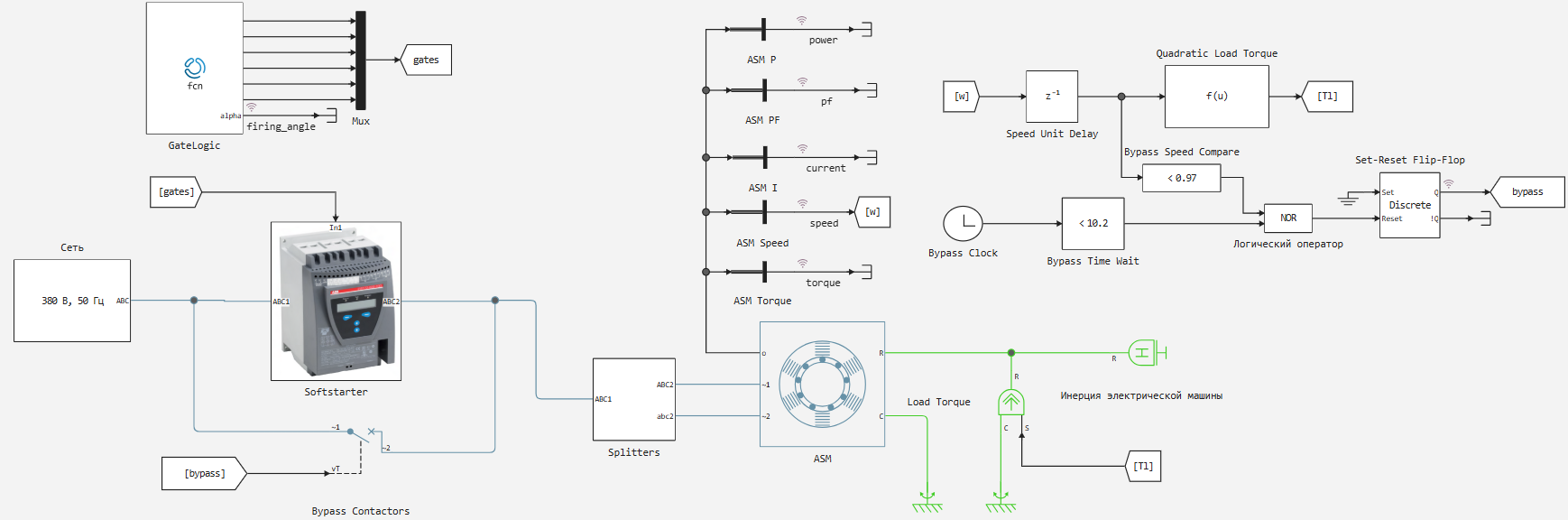
Figure 1 - Engee model of the process of overclocking an ADKZR with a fan load using an UPR
Physical blocks and load
The physical part of the model consists of the following elements.
A three-phase 380 V, 50 Hz network supplies the SCP Softstarter with six counter-parallel thyristors and RC circuits. Tripolar Bypass Contactors connected in parallel to the regulator. Asynchronous machine ASM It is connected to the "Inertia of the electric machine" unit and a controlled fan torque source. The phase sources have an amplitude of 310.269 V and shifts of 120°. A subsystem named Splitters it electrically implements a star with a common neutral.
Model management system
The branching system consists of the following parts.
The Engee Function block - GateLogic pulse routing and speed comparison logic with a threshold of 0.97 OE form the engine start and bypass.
Block Clock and a set time threshold of 10.2 s prohibits early bypass surgery of the SCP.
Blocks NOR and Set-Reset Flip-Flop they keep the contactor state.
The measuring units of the machine record the speed, torque, terminal current, active power and power factor to record the results [5, 6].
Modeling and data collection
The cell below loads the existing model file, if it is not already open, then runs engee.run. It does not cause engee.save and it does not change the parameters or blocks. After the run, the availability of the necessary keys is checked in simout. The only way to get the time series in this script is – collect(simout[ключ]) as in the example of the Engee software control [7].
In simout records are used softstarter/speed, softstarter/current, softstarter/Set-Reset Flip-Flop.Q, softstarter/GateLogic.alpha, softstarter/P_measure.1, softstarter/PF_measure.1. The measuring current of the machine is presented in relative units.
The model is designed for up to 13 with a fixed increment of 0.25 ms, that is, it has 52 001 samples per signal.
# Specify the directory where the script and the existing model are located.
ssp_project_dir = @__DIR__
model_name = "softstarter"
ssp_model_path = joinpath(ssp_project_dir,"$model_name.engee")
if !any(m -> string(m.name) == model_name, engee.get_all_models())
    engee.load(ssp_model_path)
end
# Calculating the model creates a new simout; the model file is not saved.
engee.run(model_name)
# We check that all signals for charts and bypass are recorded.
ssp_required = ["$model_name/speed","$model_name/current",
    "$model_name/Set-Reset Flip-Flop.Q","$model_name/firing_angle",
    "$model_name/power","$model_name/pf"]
ssp_missing = setdiff(ssp_required,collect(keys(simout)))
isempty(ssp_missing) || error("Нет сигналов в simout: " * join(ssp_missing,", "))
Dict(k => size(collect(simout[k]),1) for k in ssp_required)
Discussion of the results
The code in the cells below plots the speed for the entire start-up time and the current in relative units. The moment of bypass surgery it is determined by the edge of the contactor signal in simout.
using Statistics, Plots
# We read all time series only from the result of the last simout run.
ssp_speed_data = collect(simout["$model_name/speed"])
ssp_current_data = collect(simout["$model_name/current"])
ssp_bypass_data = collect(simout["$model_name/Set-Reset Flip-Flop.Q"])
ssp_power_data = collect(simout["$model_name/power"])
ssp_pf_data = collect(simout["$model_name/pf"])
ssp_t = Float64.(ssp_speed_data.time)
ssp_n = Float64.(ssp_speed_data.value)
ssp_i = Float64.(ssp_current_data.value)
ssp_b = Bool.(ssp_bypass_data.value)
# Front 1 → 0 means that the bypass contactor is closed.
ssp_edge = findfirst(ssp_b[1:end-1] .& .!ssp_b[2:end])
ssp_edge === nothing && error("Не найдено замыкание bypass")
ssp_tb = ssp_t[ssp_edge+1]
ssp_before = (ssp_t .>= ssp_tb-0.2) .& (ssp_t .< ssp_tb)
ssp_after = (ssp_t .>= ssp_tb) .& (ssp_t .< ssp_tb+0.2)
ssp_steady = ssp_t .>= 12.0
# We compare the same 0.2 s windows before and after the bypass.
ssp_stats = (; bypass_s=ssp_tb, speed_pu=mean(ssp_n[ssp_steady]),
    current_pu=mean(ssp_i[ssp_steady]),
    current_before_pu=mean(ssp_i[ssp_before]),
    current_after_pu=mean(ssp_i[ssp_after]),
    current_peak_before_pu=maximum(ssp_i[ssp_before]),
    current_peak_after_pu=maximum(ssp_i[ssp_after]),
    current_peak_start_pu=maximum(ssp_i),
    peak_change_percent=100*(maximum(ssp_i[ssp_after])/maximum(ssp_i[ssp_before])-1),
    mean_change_percent=100*(mean(ssp_i[ssp_after])/mean(ssp_i[ssp_before])-1),
    active_power_kw=mean(ssp_power_data.value[ssp_steady])*ssp_motor_and_load().S/1000,
    pf=mean(ssp_pf_data.value[ssp_steady]))
# Two graph panels: speed and current.
gr(format=:png)
ssp_p1 = plot(ssp_t,ssp_n; xlabel="Time, from", ylabel="Speed, O.E.", label="The rotor", lw=1.5)
vline!(ssp_p1,[ssp_tb]; label="Bypass", ls=:dash)
ssp_p2 = plot(ssp_t,ssp_i; xlabel="Time, from", ylabel="Current, O.E.", label="Terminal current", lw=1.4)
vline!(ssp_p2,[ssp_tb]; label="Bypass", ls=:dash)
ssp_zoom = (ssp_t .>= ssp_tb-0.2) .& (ssp_t .<= ssp_tb+0.2)
ssp_p3 = plot(ssp_t[ssp_zoom],ssp_i[ssp_zoom];
    xlabel="Time, from", ylabel="Current, O.E.", label="±0.2 s", lw=1.5)
vline!(ssp_p3,[ssp_tb]; label="Bypass", ls=:dash)
ssp_fig = plot(ssp_p1,ssp_p2, ssp_p3; layout=(3,1), size=(1000,900));

# the next line saves the graph in png
savefig(ssp_fig,joinpath(ssp_project_dir,"softstarter_script_results.png"))
# ssp_fig
The plotted graphs are shown in Figure 2.
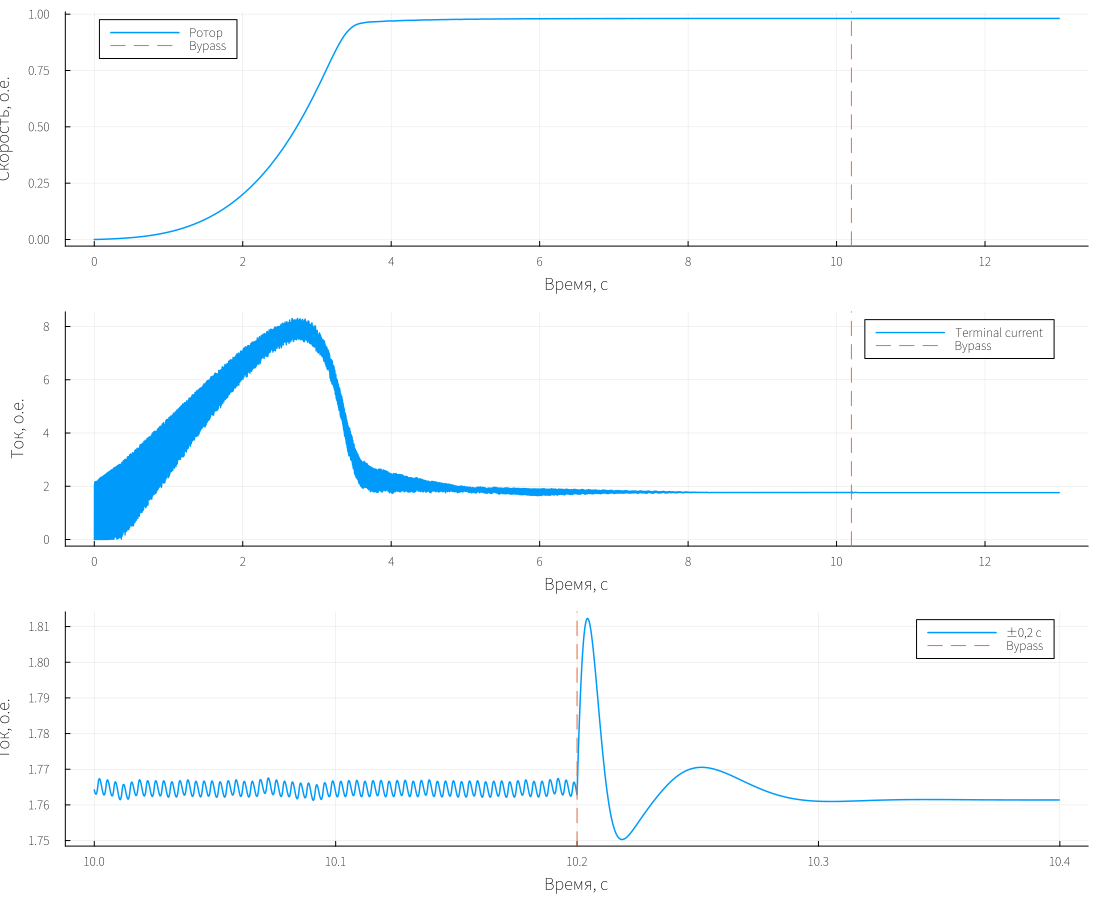
Figure 2 - Acceleration, motor current and bypass switching in the control run
During the control run, the speed after setting was 0.981 rpm, or 2942.95 rpm.
The average terminal current signal for 12-13 seconds was 1.761 ohms.;
The peak of this signal at launch is 8.303 OE, about 2.741 s.
The input active power of the engine was 16.896 kW, the power factor was 0.882.
According to the load law, the power on the fan shaft is about 15.2 kW, since the operating speed is slightly higher than the rated 2930 rpm. The indicators are summarized in table 4.
Table 4 - Benchmarks from simout
| Indicator | Meaning |
|---|---|
| Bypass closure time | 10.2 c |
| Speed after installation | 0.981 O.E. |
| Average terminal current at 12-13 c | 1.761 O.E. |
| Maximum terminal current per start | 8.303 O.E. |
| Active power after installation | 16.896 kW |
| Power factor after installation | 0.882 |
Assessment of the bypass point (bypass bypass)
Let's plot the current at the bypass point of the SCP:
ssp_zoom = (ssp_t .>= ssp_tb-0.2) .& (ssp_t .<= ssp_tb+0.2)
ssp_p3 = plot(ssp_t[ssp_zoom],ssp_i[ssp_zoom];
    xlabel="Time, from", ylabel="Current, O.E.", label="±0.2 s", lw=1.5)
vline!(ssp_p3,[ssp_tb]; label="Bypass", ls=:dash)
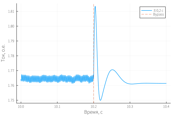
In the range of 10.0 – 10.2 s, the average terminal current is 1.764 a.e., and the maximum is 1.768 a.e.
In the range of 10.2 – 10.4 s, the average current is 1.764 OE, the maximum is 1.812 oe.
After switching, the average changed by -0.016%, the local maximum increased by 2.53%.
A brief peak is visible, but there is no steady increase in current.
The minimum speed before and after switching is 0.981 au.
Such a small dip does not disrupt acceleration. The relative changes were obtained by formula (5).
Practical recommendations and development
- Substitute the actual reduced inertia of the fan instead of the accepted one kg·m2 and check the characteristic according to the data of a specific unit.
- When selecting the SCP, check the permissible current, the number of starts per hour and the thermal load of the thyristors; there is no active current limitation in this model. For the ABB fan, it provides guidance on acceleration time and current limitation setpoint [1].
- To check the network, add a reliable impedance of the supply transformer and cable, then repeat the start at different voltages and resistance points.
- For a detailed bypass, register in phase currents and voltages on thyristors and contactor, evaluate phase matching and switching peaks.
- The script can be copied along with the model for the new engine: change the project path and passport data, recalculate the model parameters, then run and compare the metrics. You can develop it into a series of parametric runs and an automatic comparison table, keeping the reference model separate.
Used sources
- ABB. Softstarter Handbook, 1SFC132060M0201 (2010). Link.
- Pumpelprom. Technical documentation of AIR160S2. Link.
- The project "Asynchronous motor model". The Engee community.
- The block "Inertia of the electric machine". Engee documentation.
- Block "Three-phase switch and control сигнал". Engee documentation.
- Block "Measurement of asynchronous машины". Engee documentation.
- The block Software simulation management and simout". Engee documentation.
- The block Asynchronous Network Block Parameters машины". Engee documentation.