Optimization

In this example, we will demonstrate the solution of several simple optimization problems: finding the minimum of a two-parameter function using a package Optim, an explicit implementation of gradient descent and the search for an optimal solution with constraints in a linear programming problem.

Let's make a preparatory cell for loading libraries.

Pkg.add(["GLPK", "LinearAlgebra", "StatsBase", "JuMP", "Optim"])

# Загрузим необходимые библиотеки
using Plots
plotlyjs()

Plots.PlotlyJSBackend()

Optimization of the function of several variables

http://julianlsolvers.github.io/Optim.jl/v0.9.3/user/minimization/

Find the minimum of the function using the library Optim.

Specify the starting point .

using Optim
f_optim(x) = (1.0 - x[1])^2 + 100.0 * (x[2] - x[1]^2)^2
results_auto = Optim.optimize(f_optim, [0.0, 0.0])
print(results_auto)

 * Status: success

 * Candidate solution
    Final objective value:     3.525527e-09

 * Found with
    Algorithm:     Nelder-Mead

 * Convergence measures
    √(Σ(yᵢ-ȳ)²)/n ≤ 1.0e-08

 * Work counters
    Seconds run:   0  (vs limit Inf)
    Iterations:    60
    f(x) calls:    117

Implementing gradient descent

https://nextjournal.com/DeepLearningNotes/Ch06StochasticGradientDescent

The objective of this exercise is to implement a linear regression procedure through gradient descent. First, run the preparation cell.

using Plots, LinearAlgebra, StatsBase

The input data for this task is created in the following cell.

regX = rand(100)
regY = 50 .+ 100 * regX + 2 * randn(100);
scatter( regX, regY, fmt = :png, legend=:bottomright, label="data" )

The exact solution to this problem can be expressed as follows.

ϕ = hcat(regX.^0, regX.^1);
δ = 0.01;
θ = inv(ϕ'ϕ + δ^2*I)*ϕ'regY;

Let's define a quadratic loss function and calculate the gradient. After this function, we can draw a graph of the optimization function, but we will draw it at the very end of the exercise.

function loss(X,y,θ)
    cost = (y .- X*θ)'*(y .- X*θ);
    grad = - 2 * X'y + 2*X'X*θ;
    return (cost, grad)
end

loss (generic function with 1 method)

function sgd(loss, X, y, θ_start, η, n, num_iters)
    #=
       Перечень аргументов:
       loss -- функция, которую мы оптимизируем, 
               она принимает датасет (X, y) и
               текущий набор параметров θ;
               функция должна возвращать
               значение потерь и градиент при наборе параметров θ
       theta0 -- исходная оценка вектора параметров θ
       η -- шаг обучения (learning rate)
       n -- размер батча
       num_iters -- макс.количество выполнения SGD
       Возвращает:
       theta -- вектор параметров по завершению SGD
       path -- оценки оптимального θ на каждом шаге обучения
    =#
    data = [(X[i,:],y[i]) for i in 1:length(y)]
    θ = θ_start
    path = θ
    for iter in 1:num_iters
        s = StatsBase.sample(data, n)
        Xs = hcat(first.(s)...)'
        ys = last.(s)
        cost, grad = loss(Xs,ys,θ)
        θ = θ .- ( ( η * num_iters/(num_iters+iter) * grad) / n )
        path = hcat(path,θ)
    end
    return (θ,path)
end

sgd (generic function with 1 method)

Graph output with optimization progress:

# Поверхность функции потерь
xr = range(40, stop=60, length=10);
yr = range(90, stop=110, length=10);
X = hcat(ones(length(regX)), regX);
f(x,y) = loss(X,regY,[x y]')[1][1];
plot(xr, yr, f, st=:wireframe, fmt = :png, label="Функция потерь", color="blue")

# Пути оптимизации
X = hcat(ones(length(regX)), regX);
y = regY;
(t,p) = sgd(loss, X, y, [40 90]', 0.1, 1, 500);
scatter!( p[1,:], p[2,:], f.(p[1,:],p[2,:]),
    label="Путь оптимизации", ms=3, markerstrokecolor = "white", camera=(40,30) )

Let's output the optimization results:

println("Координаты найденной точки, в которой функция принимает минимальное значение:")
print( p[:,end] )

Координаты найденной точки, в которой функция принимает минимальное значение:
[50.44203686443982, 99.09098067162014]

Finding the optimal solution with constraints

https://www.juliabloggers.com/optimization-with-jump-in-julia/

Suppose we are faced with such an optimization problem:

The range of acceptable values is shown in the figure (x and y are continuous, independent variables):

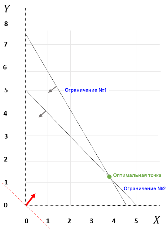
We are given an optimization objective (red arrow) and a direction (maximization), the green dot is the optimal solution, its coordinates are x = 3.75 and y = 1.25. The optimal value of the objective function is 23.75.

Let's solve this problem using the JuMP library Julia for optimization.

using JuMP, GLPK

# Зададим модель
m = Model(); # m будет значить "модель"

# Выберем оптимизатор
set_optimizer(m, GLPK.Optimizer); # выберем решатель GLPK (GNU Linear Programming Kit)

# Определим
@variable(m, x>=0);
@variable(m, y>=0);

# Определим ограничения
@constraint(m, x+y<=5);
@constraint(m, 10x+6y<=45);

# Определим целевую функцию
@objective(m, Max, 5x+4y);

# Запустим решатель
optimize!(m);

# Вывод
println(objective_value(m)) # Значение целевой функции в оптимальной точке
println("x = ", value.(x), "\n","y = ",value.(y)) # Координаты оптимальных x и y

[ Info: Precompiling JuMP [4076af6c-e467-56ae-b986-b466b2749572]
[ Info: Precompiling GLPK [60bf3e95-4087-53dc-ae20-288a0d20c6a6]

23.75
x = 3.75
y = 1.2500000000000002