The Van der Pol oscillator
In this example, we will show how to create a dynamics model in Engee that works according to the second-order Van der Pol equation.
Introduction
The Van der Pol oscillator demonstrates the dynamics of not консервативной systems with nonlinear attenuation.
This system can be described by the following equation:
where – coordinate (for example, the position of the oscillator), – damping coefficient. This model is used to study a wide variety of processes in biology and physics, including radio engineering and electronics.
We will model this system using blocks on a canvas for graphical modeling in Engee. In the file van_der_pol_oscillator.engee contains a model of the following type:
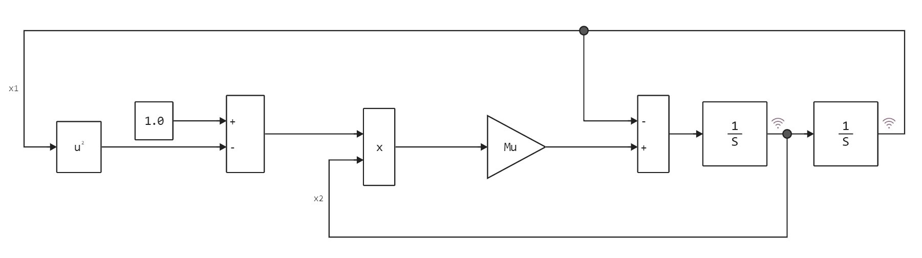
It has two separate integrators that are responsible for calculating the signals. x1 (coordinate) and x2 (speed).
Starting the model with μ = 1
If you run this model with the argument then we will see an auto-oscillatory mode of operation with nonlinear attenuation. Loading the model:
if "van_der_pol_oscillator" in [m.name for m in engee.get_all_models()]
    m = engee.open( "van_der_pol_oscillator" );
else
    m = engee.load( "/user/start/examples/edu/van_der_pol_oscillator/van_der_pol_oscillator.engee" );
end
Let's run the model in its original form and build a graph.:
data = engee.run( m );

plot( data["x1"].value, data["x2"].value )
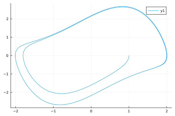
We can choose different starting points, changing the initial value of each integrator, but the system will always come to the limit cycle.
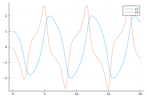
You can build a graph for each signal separately.
plot( data["x1"].time, data["x1"].value, label="x1" )
plot!( data["x2"].time, data["x2"].value, label="x2" )
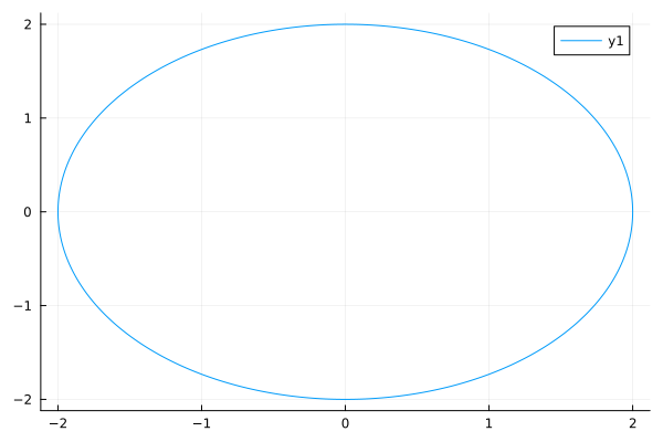
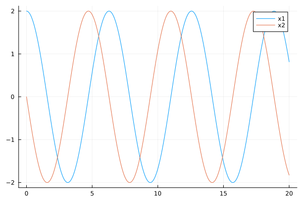
Starting the model with μ = 0
In this mode, the equation of the system is reduced to the equation of a conventional harmonic oscillator.:
Let's set the coefficient set to zero and run the model.
engee.set_param!( "van_der_pol_oscillator/Mu", "Gain"=>0 )

data = engee.run( m );
data = engee.run( m );

using Plots
plot( data["x1"].value, data["x2"].value )
Let's build another graph for this system.:
plot( data["x1"].time, data["x1"].value, label="x1" )
plot!( data["x2"].time, data["x2"].value, label="x2" )
Conclusion
We have seen that graphical modeling in Engee is a convenient way to experiment with the topology of the system, complicate the model, or use it as part of a complex demonstration.