Numerical integration
In this example, we will learn how to integrate a vector of velocity measurements and make a conclusion about the distance traveled.
Let's study the initial data
Let's assume that we have a vector of car speed measurements taken at different points in time.
vel = [ 0, .45, 1.79, 4.02, 7.15, 11.18, 16.09, 21.90, 29.05, 29.05,
        29.05, 29.05, 29.05, 22.42, 17.9, 17.9, 17.9, 17.9, 14.34, 11.01,
        8.9, 6.54, 2.03, 0.55, 0 ];
vTime = 0:24;
The data is recorded at regular intervals (every second, 24 seconds in a row). Let's output a graph of the observed process:
gr()
plot( vTime, vel, title="Vehicle speed", markershape=:star8,
      xlabel="Time, from", ylabel = "Speed, m/s", legend=false )
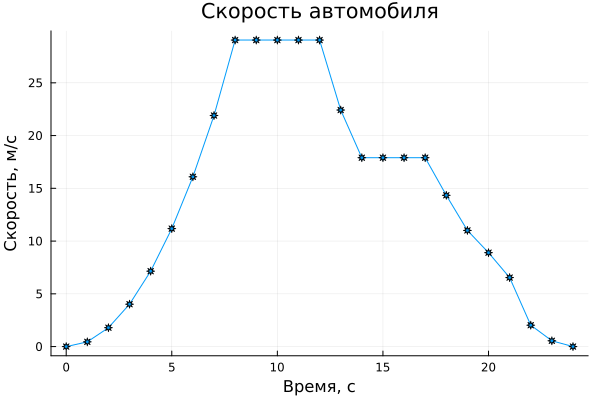
A positive slope corresponds to the intervals when the car was accelerating, a flat horizontal graph corresponds to moving at a constant speed, and a negative slope corresponds to braking intervals. At a moment in time t=0 the car was stationary, the speed at that moment was 0 m/ s. The car accelerated to reach a maximum speed of 29.05 m/s at approximately t=8. She maintained this speed for 4 seconds. Then she began to slow down to 17.9, held this speed for three seconds, and continued to slow down unevenly until she came to a complete stop.
It is difficult to describe this curve with a single continuous function, since it has many discontinuities of the derivative.
Calculate the distance traveled
For numerical integration, we will use the package Trapz, which can be set as follows:
]add Trapz
Function trapz integrates a discrete time series using the trapezoid method from this package. This method is well suited for data with clearly observed discontinuities and assumes that the dynamics of the system changed linearly between two points.
To illustrate the idea of this method, let's draw several trapezoids on a graph with our data.:
plot( vTime, vel, title="Vehicle speed", markershape=:star8,
      xlabel="Time, from", ylabel = "Speed, m/s", legend=false )
plot!( vTime, vel, fillrange=zeros(length(vel)), fillcolor=:blue, label=:none, lw=2, lc=:black )
for i in 1:length(vTime)
    plot!( [vTime[i],vTime[i]], [0,vel[i]], lw=2, lc=:black )
end
plot!()
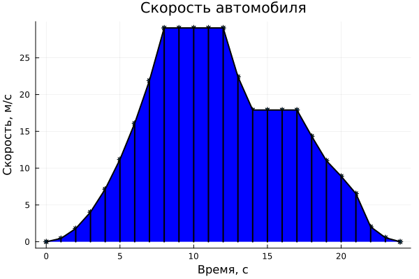
Function trapz allows you to calculate the area under any piecewise linear curve, using the sum of the areas of the trapezoids under each interval.
Let's calculate the distance traveled by the car during the observation (the area of the entire shaded area on the graph) using numerical integration.
using Trapz
distance = trapz( vTime, vel )
So, in 24 seconds, the car overcame 345.22 m.
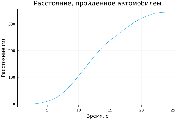
Let's display a graph of the distance traveled
In the library NumericalIntegration There is another feature that will be useful to us. – cumul_integrate.
]add NumericalIntegration
Function cumul_integrate It also performs numerical integration, but returns not the area under the entire curve, but the accumulated amount at each observation point of the initial value.
using NumericalIntegration: cumul_integrate
cdistance = cumul_integrate( vTime, vel );
We have calculated how much of the distance the car traveled from the beginning to each timestamp, now we will build a graph.
plot( cdistance, title = "Distance traveled by car",
      xlabel = "Time, from", ylabel = "Distance (m)", legend=false )
Conclusion
We applied a couple of simple functions to integrate discrete time series (the vector of measured velocity) and obtained the distance traveled during the entire observation period and a graph of how to overcome this for each time interval.