Mathematical statistics
In this example, we will demonstrate how to solve simple problems in the field of mathematical statistics – obtaining a series of random numbers, modeling a discrete distribution, constructing a probability density of a normally distributed random variable, and an example of Kalman filtering.
First, perform the preparatory cells to set up the graph rendering.
Pkg.add(["Distributions", "LinearAlgebra", "StatsBase", "Measures"])
using LaTeXStrings;
using Plots

gr()
# plotlyjs(); # For interactive graphs
Implementation of a random variable
Task: Display one hundred points from the normal distribution of a random variable with a variance of 1 and a mathematical expectation of -2.
n = 100;
ϵ = randn(n) .- 2;
plot(1:n, ϵ, label=L"\mathcal{N}(-2, 1)")

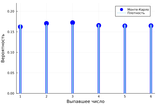
Discrete distribution: playing dice
Task: Compare two distributions of a random variable that describes the result of rolling one hexagonal die, obtained by the Monte Carlo method and through the library Distributions.
using Distributions, StatsBase, Plots;

faces, N = 1:6, 10^4
mcEstimate = counts(rand(faces,N), faces)/N

a = Distributions.DiscreteUniform(1,6)

plot(faces, mcEstimate, line=:stem, marker=:circle, c=:blue,
    ms=10, msw=0, lw=8, label="Monte Carlo", xticks=1:12, )

plot!([i for i in faces], [pdf(a, x) for x in faces], line=:stem, label="Density",
    lw=5, lc=:skyblue,
    xlabel="The dropped number", ylabel="Probability", ylims=(0,0.22))
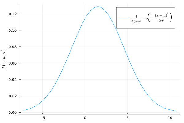
Probability density of a normal random variable
Task: Plot the probability density of a distribution with a mathematical expectation of 1.5 and a variance of 3.1.
using Distributions, Plots, LaTeXStrings
d = Normal(1.5, 3.1)

x = sort!(rand(d,1000))
y = pdf.(d, x)

plot(x, y, label=L"\frac{1}{\sqrt{2 \pi \sigma^2}} \exp \left( - \frac{(x - \mu)^2}{2 \sigma^2} \right)")
ylabel!(L"f(x; \mu, \sigma)")
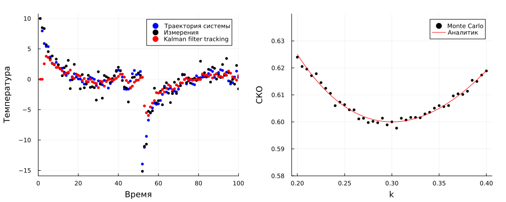
One-dimensional example of Kalman filtering [1,p.343]
Many systems of physical nature can be described using a model of the following form:
The gain matrices in the Kalman filter can be calculated iteratively to improve filtering results. In this example, all variables are scalar quantities. We believe that and the model tends to 0 with force at every moment of time.
Task: Demonstrate the Kalman filter's ability to track a one-dimensional autoregressive process.
using Distributions, LinearAlgebra, Random, Measures, Plots;
Random.seed!(1)

a, varXi, varZeta, = 0.8, 0.36, 1.0
X0, spikeTime, spikeSize = 10.0, 50, -20.0
Tsmall, Tlarge, warmTime = 100, 10^6, 10^4
kKalman = 0.3

function luenbergerTrack(k, T, spikeTime = Inf)
    X, Xhat = X0, 0.0
    xTraj, xHatTraj, yTraj = [X], [Xhat,Xhat], [X0]

    for t in 1:T-1
        X = a*X + rand(Normal(0,sqrt(varXi)))
        Y = X + rand(Normal(0,sqrt(varZeta)))
        Xhat =a*Xhat - k*(Xhat - Y)

        push!(xTraj,X)
        push!(xHatTraj,Xhat)
        push!(yTraj,Y)

        if t == spikeTime
            X += spikeSize
        end
    end
    deleteat!(xHatTraj,length(xHatTraj))
    xTraj, xHatTraj, yTraj
end

smallTraj, smallHat, smallY = luenbergerTrack(kKalman, Tsmall, spikeTime)

p1 = scatter(smallTraj, c=:blue, ms=3, msw=0, label="Trajectory of the system")
p1 = scatter!(smallY, c = :black, ms=3, msw=0, label="Measurements")
p1 = scatter!(smallHat,c=:red, ms=3, msw=0, label="Kalman filter tracking",
xlabel = "Time", ylabel = "Temperature", xlims=(0, Tsmall))

kRange = 0.2:0.005:0.4
errs = []
for k in kRange
    xTraj, xHatTraj, _ = luenbergerTrack(k, Tlarge)
    mse = norm(xTraj[warmTime:end] - xHatTraj[warmTime:end])^2/(Tlarge-warmTime)
    push!(errs, mse)
end

analyticErr(k) = (varXi + k^2*varZeta) / (1-(a-k)^2)

p2 = scatter(kRange,errs, c=:black, ms=3, msw=0,
xlabel="k", ylabel="SKO", label = "Monte Carlo")
p2 = plot!(kRange,analyticErr.(kRange), c = :red,
xlabel="k", ylabel="SKO", label = "Analyst", ylim =(0.58,0.64))

plot(p1, p2, size=(1000,400), margin = 5mm)