The three-body problem
We implement a numerical solution to the problem of simulating the dynamics of three bodies in gravitational interaction with each other.
Task description
Three material points with coordinates , , and speeds , , they are located in a single space. It is necessary to determine their trajectories in time.
As we know, unfortunately, there is no analytical solution to the problem of calculating the coordinates of all objects in the system at any given time. t. But we will solve this problem using numerical integration.
Here, the radius vectors of each body are denoted., – their second derivatives (acceleration), – the mass of each body, the gravitational constant It can be assumed to be equal to 1 without loss for our needs to visualize the dynamics of the system. Designation It implies the norm between radius vectors, in other words, the distance between bodies 1 and 2.
So, the gravity of each of the two bodies affects the acceleration of the third. We have formulated equations for which there is no analytical solution, moreover, when our solution will be abstract and will not have the right dimensions.
Solving a system of differential equations
To solve this system of three second-order differential equations, we will also need to solve first-order equations. Let's use the library DifferentialEquations:
Pkg.add(["DifferentialEquations"])
using DifferentialEquations
gr()
julia = Colors.JULIA_LOGO_COLORS # Let the graphics be in the colors of the Julia logo.
Solving the current step and updating the system status, we will create a function thereebody.
function threebody( du, u, p, t )
    # Position, speed
    x1, y1, x2, y2, x3, y3,
    vx1, vy1, vx2, vy2, vx3, vy3 = u

    # System parameters (weight of each body)
    m1, m2, m3 = p

    # Increment of coordinates of each body
    du[1] = vx1; du[2] = vy1; du[3] = vx2; du[4] = vy2; du[5] = vx3; du[6] = vy3;

    # The distance from one body to another
    r12 = sqrt((x1 - x2) ^ 2 + (y1 - y2)^2 )
    r23 = sqrt((x2 - x3) ^ 2 + (y2 - y3)^2 )
    r13 = sqrt((x1 - x3) ^ 2 + (y1 - y3)^2 )

    # Acceleration (at G=1)
    du[7]  = -m2 * ((x1-x2) / (r12^3)) - m3 * ((x1-x3) / (r13^3))
    du[8]  = -m2 * ((y1-y2) / (r12^3)) - m3 * ((y1-y3) / (r13^3))

    du[9]  = -m3 * ((x2-x3) / (r23^3)) - m1 * ((x2-x1) / (r12^3))
    du[10] = -m3 * ((y2-y3) / (r23^3)) - m1 * ((y2-y1) / (r12^3))

    du[11] = -m1 * ((x3-x1) / (r13^3)) - m2 * ((x3-x2) / (r23^3))
    du[12] = -m1 * ((y3-y1) / (r13^3)) - m2 * ((y3-y2) / (r23^3))

end
You can see that vectorization would significantly shorten our code, as well as using the function norm() from the library LinearAlgebra to calculate the distances. But in this tutorial, for now, we will give preference to the visual similarity of the code and formulas, which is in the current implementation.
Setting the initial parameters
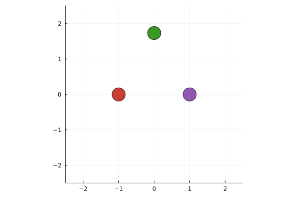
We have a large vector of initial coordinates. We will add several input fields to make it easy to change these parameters.
We will use the following numbers (in one direction or another) as the initial velocity values:
Remark:
1) The next cell is not executed automatically, to update the values of the variables, press the ⏵ button, or click in the free area of the mask and launch the cell using the keyboard shortcut Ctrl+Enter.
2) To hide the code and leave only the controls, double-click on the mask.
# @markdown # Starting position $\bar x_1 \dots \bar x_3$

Положение_по_умолчанию = false # @param {type: "boolean"}
if there is a silence clause
    x1_0 = -1.0
    y1_0 =  0.0
    x2_0 =  1.0
    y2_0 =  0.0
    x3_0 =  0.0
    y3_0 =  sqrt(3)
else
    x1_0 = -1.0   # @param {type:"slider", min:-2, max:2, step:0.1}
    y1_0 =  0.0   # @param {type:"slider", min:-2, max:2, step:0.1}
    x2_0 =  1.0   # @param {type:"slider", min:-2, max:2, step:0.1}
    y2_0 =  0.0   # @param {type:"slider", min:-2, max:2, step:0.1}
    x3_0 =  0.0   # @param {type:"slider", min:-2, max:2, step:0.1}
    y3_0 =  1.732 # @param {type:"slider", min:-2, max:2, step:0.1}
end
scatter( [x1_0, x2_0, x3_0],
         [y1_0, y2_0, y3_0],
         mc=[julia.red, julia.purple, julia.green],
         ms=15, xlimits=(-2.5,2.5),
         ylimits=(-2.5,2.5),
         legend=:none, aspect_ratio=:equal )
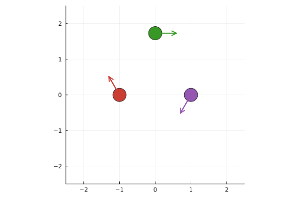
# @markdown # Initial velocity $\bar v_1 \dots \bar v_3$
# @markdown
Скорость_по_умолчанию = false # @param {type: "boolean"}
if the speed is silent
    vx1_0, vy1_0, vx2_0, vy2_0, vx3_0, vy3_0 =
       0.074, 0.128, -0.074, -0.128, 0.148, 0.0
else

    vx1_0 = -0.074  # @param {type:"slider", min:-1.0, max:1.0, step:0.001}
    vy1_0 = 0.128  # @param {type:"slider", min:-1.0, max:1.0, step:0.001}
    vx2_0 = -0.074  # @param {type:"slider", min:-1.0, max:1.0, step:0.001}
    vy2_0 = -0.128  # @param {type:"slider", min:-1.0, max:1.0, step:0.001}
    vx3_0 =  0.148  # @param {type:"slider", min:-1.0, max:1.0, step:0.001}
    vy3_0 =  0.0    # @param {type:"slider", min:-1.0, max:1.0, step:0.001}
end

scatter( [x1_0, x2_0, x3_0], [y1_0, y2_0, y3_0],
mc=[julia.red, julia.purple, julia.green], ms=15, xlimits=(-2.5,2.5), ylimits=(-2.5,2.5),
         legend=:none, aspect_ratio=:equal )

plot!( [x1_0, x1_0+4*vx1_0], [y1_0, y1_0+4*vy1_0], c=julia.red, lw=2, arrow=true )
plot!( [x2_0, x2_0+4*vx2_0], [y2_0, y2_0+4*vy2_0], c=julia.purple, lw=2, arrow=true )
plot!( [x3_0, x3_0+4*vx3_0], [y3_0, y3_0+4*vy3_0], c=julia.green, lw=2, arrow=true )
# @markdown # Parameters of $\bar m_1 \dots \bar m_3$
# @markdown
Масса_по_умолчанию = false # @param {type: "boolean"}
if the mass is silent
    m1, m2, m3 = 0.1, 0.1, 0.1
else
    m1 = 0.1  # @param {type:"slider", min:0.01, max:2.0, step:0.01}
    m2 = 0.1  # @param {type:"slider", min:0.01, max:2.0, step:0.01}
    m3 = 0.1  # @param {type:"slider", min:0.01, max:2.0, step:0.01}
end
;
# @markdown # Simulation duration
# @markdown
t_begin = 0
t_end =   100.0  # @param {type:"number"}
;
Let's formulate the problem and solve the system of odes
# Let's put all the initial values of the variables into vectors
p = [m1, m2, m3]
u_begin = [ x1_0, y1_0, x2_0, y2_0, x3_0, y3_0,
            vx1_0, vy1_0, vx2_0, vy2_0, vx3_0, vy3_0 ];
t_span = (t_begin, t_end)

# Let's formulate the problem to be solved
prob = ODEProblem( threebody, u_begin, t_span, p )

# We get the solution
sol = solve( prob, Vern7(), reltol = 1e-16, abstol=1e-16 );
Auxiliary code for displaying graphs
Let's create a function that will extract individual trajectories from the solution that we received.
function get_values( sol; dt = 0.001, final = 1.0 )

    final_time = sol.t[end] * final;

    idx = sol.t[1]:dt:final_time

    x1_values = map( value -> value[1], sol.(idx) )
    y1_values = map( value -> value[2], sol.(idx) )
    x2_values = map( value -> value[3], sol.(idx) )
    y2_values = map( value -> value[4], sol.(idx) )
    x3_values = map( value -> value[5], sol.(idx) )
    y3_values = map( value -> value[6], sol.(idx) )

    return(
        [x1_values, x2_values, x3_values],
        [y1_values, y2_values, y3_values]
    )

end
This function will allow us to decompose the variables from the solution. sol into several vectors, where the coordinates will be collected x and y.
x_values, y_values = get_values(sol);
Let's create a few more variables that will contain the position of each body at the end of the simulation.
x1_end = x_values[1][end]; y1_end = y_values[1][end];
x2_end = x_values[2][end]; y2_end = y_values[2][end];
x3_end = x_values[3][end]; y3_end = y_values[3][end];
Let's deduce the solution
You can directly plot all the coordinates individually and estimate where the objects are located, but this graph will be confusing and will take up a lot of space in the file (about 40 MB).
# plot( sol )
Instead, we will display several other graphs.
traj = plot( x_values, y_values,
             c=[julia.red julia.purple julia.green],
             legend=false,
             title="The three-body problem",
             xaxis="X", yaxis="Y",
             xlims=(-2.0, 2.0),
             ylims=(-1.0, 2.0),
             aspect_ratio = 1.1 )
scatter!( traj, [x1_end, x2_end, x3_end], [y1_end, y2_end, y3_end],
          mc=[julia.red, julia.purple, julia.green], ms=7 )
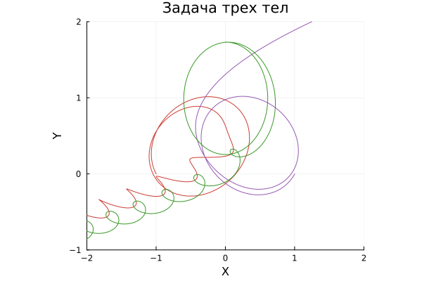
The most common outcome of this experiment is that one of the bodies separates from the others, while the other two form a binary system and continue to move in space around a common center of gravity.
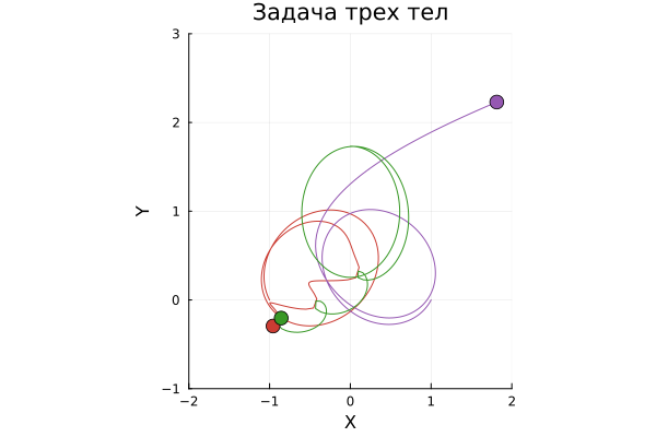
To better study the movement of bodies, we will build an interactive simulation.
# @markdown # Model time
# @markdown
time_fraction = 0.307  # @param {type:"slider", min:0.0, max:1.0, step:0.001}

x_values, y_values = get_values(sol, dt=0.1, final=time_fraction);

x1_end = x_values[1][end]; y1_end = y_values[1][end];
x2_end = x_values[2][end]; y2_end = y_values[2][end];
x3_end = x_values[3][end]; y3_end = y_values[3][end];

traj = plot( x_values, y_values,
             c=[julia.red julia.purple julia.green],
             legend=false,
             title="The three-body problem",
             xaxis="X", yaxis="Y",
             xlims=(-2.0, 2.0),
             ylims=(-1.0, 3.0),
             aspect_ratio = 1.1 )
scatter!( traj, [x1_end, x2_end, x3_end], [y1_end, y2_end, y3_end],
          mc=[julia.red, julia.purple, julia.green], ms=7 )
Conclusion
We built a model of a system of three material points and at the same time showed how masking code cells allows us to control the parameters and solution of this differential system over time.
You can easily check that the smallest change in the model parameters (coordinates, velocity, or mass) This leads to a huge change in the final trajectories, which is the main feature of chaotic systems.