The Fibonacci Spiral
In this example, we will look at how to use interactive scripts to conveniently compare the results of different models – graphical and those specified as a text program.
We will build a graphical model that generates points on the Fibonacci spiral, and then compare the resulting graph with the result of calculating the golden spiral model.
The object under study
The Fibonacci spiral is an approximation of the golden spiral. It was described by Leonardo of Pisa (nicknamed Fibonacci) around 1202. It is defined using a piecewise linear curve consisting of quarters of circles. The radius of each quarter circle It is set by a recurrence relation that forms the famous Fibonacci sequence.:
where .
(the first two terms 0, 1 are usually discarded, the spiral is built immediately from the third term: 1, 2, 3, 5, 7...)< br>
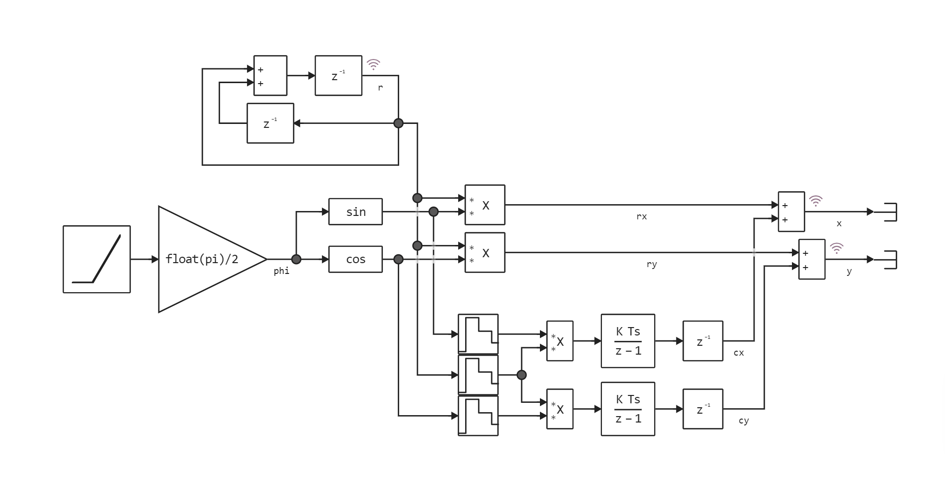
The center of each circle is selected so that the spiral remains smooth. The points of the center of each circle can be obtained from the model fibonacci_spiral_model.engee (signals cx and cy) along with their radii (signals r). By output signals x and y We will plot the Fibonacci spiral chart.
The general view of the model is presented below:
The Golden Spiral
The golden spiral is defined on the entire numeric axis using a single exponential function. This function is equally simple to set using both a mathematical expression and a graphical model. We are talking about a logarithmic spiral, the radix of which is for every half revolution , increases by the value . Here – the number that is the inverse of the golden ratio .
We will have to complicate the usual logarithmic spiral equation. . The point is that the convergence point The Fibonacci spiral is not located at the origin and depends on the size of the rectangle in which the Fibonacci spiral is inscribed. To match both spirals, you also need to enter a non-zero angle of initial rotation into the golden spiral equation. .
For the derivation of the formula of the golden spiral, which maximally coincides with the Fibonacci spiral, it is better to refer to the publication [1]. Here we will only give the final formula of the golden spiral in polar coordinates.:
where – a series of coordinates of points on a spiral in the polar coordinate system, – the width of the rectangle in which the Fibonacci spiral is inscribed.
Launching the model
Let's launch the model fibonacci_spiral_model.engee and let's analyze the results.
modelName = "fibonacci_spiral_model";
model = modelName in [m.name for m in engee.get_all_models()] ? engee.open( modelName ) : engee.load( "$(@__DIR__)/$(modelName).engee");
This design allowed us to check if the model was uploaded and opened by the user (then we need the command open), or you need to download it using the command load.
It is very easy to run the model:
s = engee.run( modelName, verbose=false )
Output object s it contains tables with those signals that are marked as "logged" in the model (using the icon ).
Analysis of the results
Let's choose an environment for drawing graphs.
gr() # Static graphs of small size
# plotly() # Interactive graphs by screen width
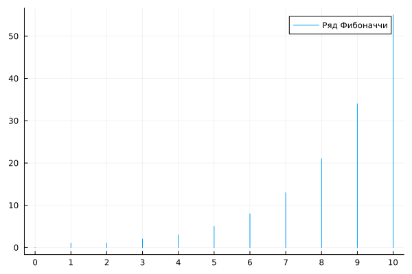
Visualize a series of Fibonacci numbers: the signal r. This vector contains quite a few points, because the model generating them has a low sampling rate.
plot( s["r"].time, s["r"].value, label="Fibonacci Series", st=:stem )

# Setting our own signatures for the X scale
plot!( xticks=( range( minimum(s["r"].time), maximum(s["r"].time), step=1),
           Int.(range( minimum(s["r"].time), maximum(s["r"].time), step=1))) )
Building the Golden Spiral
As we discussed, in order to build a golden spiral that matches the Fibonacci spiral, we first need to get several parameters from an already constructed spiral.
theta = range( -0.8*pi, 12*pi, step=0.01); # The scope of the Golden spiral definition

λ = (sqrt(5)-1)/2; # The number that is the reverse of the golden ratio

# The dimensions of the rectangle in which the Fibonacci spiral is inscribed
a = maximum(s["x"].value) - minimum(s["x"].value)
b = maximum(s["y"].value) - minimum(s["y"].value)

# Coordinates of the center of the Fibonacci spiral
# - in the coordinate system of this rectangle)
x = (1 - λ)/(2 - λ) * a
y = (1 - λ)/(2 - λ) * b
# - in the coordinate system of the graph
sx = minimum(s["x"].value) + x;
sy = maximum(s["y"].value) - y; # (note that the y-axis is pointing upwards)

# The angle of rotation of the golden spiral relative to the Fibonacci spiral
α = atan( 2*λ - 1 );
Now you can calculate the coordinates of the points lying on the golden spiral.
# Points of the golden spiral in the polar coordinate system
R = @. (a/(2 - λ)) * sqrt(1 + λ^6) * λ^((2/pi)*(theta+α))
# The points of the golden spiral in the Cartesian coordinate system
x,y =  R .* cos.( theta ) .+ sx, R .* sin.( theta ) .+ sy;
It remains to display both graphs for visual comparison.
plot( s["x"].value, s["y"].value, lc=:skyblue, aspect_ratio=:equal, lw=4, label="The Fibonacci Spiral" )
plot!( x, y, lc=:black, ls=:dash, label="The Golden Spiral", legend=:topleft )
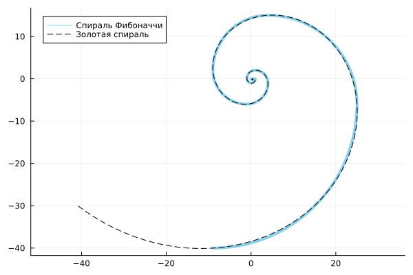
Obviously, the models match up pretty well.
Conclusions
We used the basic blocks of Engee to build a mathematical model that approximates the golden spiral. Then, using software control commands, we visualized several signals and compared the result with the golden spiral equation.
Link:
[1] Duan J. S. Shrinkage points of golden rectangle, Fibonacci spirals, and golden spirals //Discrete Dynamics in Nature and Society. – 2019. – Vol. 2019. – pp. 1-6.