Building Lissajous curves
Modeling basic mathematical objects helps to better understand the work of the processes that generate them. In this example, we will explore two ways to build models that create Lissajous figures, as well as configure these models and compare their operation using the program management commands described on the documentation page "Software simulation management".
The simulated process
Lissajous figures are tracks drawn by a point that performs two harmonic vibrations simultaneously. They are usually generated using a system of two trigonometric functions. Dependence of coordinates and from time to time it has the following form:
here – the amplitudes of each harmonic process (we will have equal 1)
– the frequencies of both processes,
– the shift between harmonic processes.
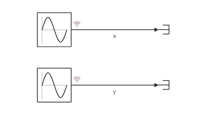
A model created from sinusoid generators
Our first model will consist of two blocks Sine Wave.
The model specified as a code
The second model will consist of one block Engee Function and several blocks Constant, setting the system parameters we are interested in.
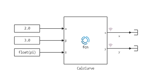
In both cases, the output parameters are the signals x and y, and they are marked as logable signal. Thanks to this, we will be able to count them when the simulation is started programmatically.
Loading models
The first step is to get control of these models. When the model is already open (for example, it is on the canvas), one command is used for this, when it needs to be loaded, another command is needed. Getting a list of uploaded models:
all_model_names = [m.name for m in engee.get_all_models()]
If the model is already open, then we use the function open to get control for a few days. If not, we will use the function load.
# A model consisting of blocks
if "lissajous_curve_blocks" in all_model_names m1 = engee.open( "lissajous_curve_blocks" )
else m1 = engee.load( "$(@__DIR__)/lissajous_curve_blocks.engee" )
end;

# A model consisting of the code
if "lissajous_curve_function" in all_model_names m2 = engee.open( "lissajous_curve_function" )
else m2 = engee.load( "$(@__DIR__)/lissajous_curve_function.engee" )
end;
Now we have two objects., m1 and m2 through which we can control the parameters and operation of both models we are studying.
Synchronization of model parameters
From the ratio of the parameters and the shape of the curve (the number of petals) depends. Now we will set the same parameters for both models using software control commands. We want the models to use the following parameters:
alpha = 3;
beta = 4;
Let's study the structure of the block parameters Sine Wave models lissajous_curve_blocks.
param = engee.get_param( "lissajous_curve_blocks/Sine Wave" )
This is a type structure Pair, which can be changed and passed in its entirety as new block parameters lissajous_curve_blocks/Sine Wave:
param["Frequency"] = string(alpha)
engee.set_param!( "lissajous_curve_blocks/Sine Wave", param... )
You can also use a shorter syntax. Let's do the same for the second block and for the second model.:
engee.set_param!( "lissajous_curve_blocks/Sine Wave-1", "Frequency"=>string(beta) )
engee.set_param!( "lissajous_curve_function/Constant", "Value"=>string(alpha) )
engee.set_param!( "lissajous_curve_function/Constant-1", "Value"=>string(beta) )
The structure of the simulation parameters can be obtained by the command engee.get_param( "lissajous_curve_function" ).
We will set the same simulation step for both models.:
param = engee.get_param( "lissajous_curve_blocks" )
# We will set a time step of 0.001 for both models.
engee.set_param!( "lissajous_curve_function", "FixedStep"=>"0.001" )
engee.set_param!( "lissajous_curve_blocks", "FixedStep"=>"0.001" )
Now we can execute these models using the command run:
r1 = engee.run( m1; verbose=false );

# Sometimes you need to wait for the model to finish executing.
# while( engee.get_status() != Engee.Types.READY ) end;
r2 = engee.run( m2; verbose=false )
At the output, we get the structure Dict (dictionary), which contains a set of tables DataFrame. Each table has vector columns time and value, corresponding to the time and output value of each stored model signal.
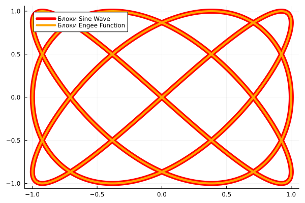
Simulation results
The output curves are easy to compare using a graph.:
plot( r1["x"].value, r1["y"].value, lc=:red, lw=10, label="Sine Wave Blocks" )
plot!( r2["x"].value, r2["y"].value, lc=:orange, lw=4, label="Engee Function Blocks" )
Conclusions
We have studied the operation of two models of one of the basic mathematical objects, which is considered in a wide variety of technical disciplines – from physics to circuit engineering. We also applied the program control mechanism, setting the same parameters for the models and analyzing the simulation results on the graph without leaving the script.