Flappy Bird AI: Evolutionary learning of neural networks on Julia

Flappy Bird is an iconic mobile game that has become an ideal testing ground for demonstrating the principles of machine learning due to its simplicity and clear rules. In this project, we have implemented not only the game itself, but also two different neural network architectures that are trained to play it using an evolutionary algorithm.

Key features of the project:

Full implementation on the Julia standard library without external dependencies
Symbolic rendering of the game in the terminal
Two neural network architectures: fully connected (DenseNet) and convolutional (CNN)
A genetic algorithm for learning
Interactive menu for managing training and testing

The project demonstrates how, even using only the basic features of a programming language, it is possible to create a full-fledged machine learning system. Flappy Bird was not chosen by chance — it is an ideal testbed.:

Simple rules, but difficult skill
Clear reward system (points for flying through pipes)
Discrete actions (jump or not)
Visually understandable learning progress

Using symbolic graphics on the command line shows that complex graphics libraries are not needed to demonstrate machine learning concepts — the algorithms and principles themselves are important.

Technology stack:

Julia as a high-performance language for scientific computing
Genetic algorithms as a gradient-free optimization method
Neural networks as universal approximators
Console interface for maximum portability

This project aims to show "from the inside" how neural networks and evolutionary algorithms work, without the magic of deep learning frameworks.

Now let's move on to the actual implementation of the project. The Flappy Bird implementation is based on two key data structures that encapsulate the state of all game objects, and a set of global parameters that determine the physics and balance of the game. This minimalistic approach is typical for game engines, where a clear separation of data and logic ensures predictability and ease of debugging.

The Bird object is a controlled bird, the main character of the game. Its fields store the full dynamic state: the vertical position y (a fractional number for smoothness), the speed v (positive down, negative up), the current score s (an integer number of pipes passed) and the Boolean activity flag a, indicating whether the bird is alive. These four parameters are sufficient to describe the entire mechanics of a bird's movement — its reaction to gravity, the impulse to jump, and interaction with boundaries.

Each pipe is represented by a Pipe structure containing three parameters: the horizontal x coordinate (tracks the position of the pipe relative to the bird), the vertical passage position gy (determines where the safe gap is) and the passage flag p (eliminates repeated scoring). The pipes move towards the bird, creating the main challenge of the game — the need to accurately fly through narrow gaps.

The GP array contains seven numeric constants that define the geometry and physics of the game world. These are the width and height of the field, the force of gravity and jumping, the size of the pipes, as well as the speed of their movement. This centralized configuration makes it easy to balance the complexity of the game and experiment with parameters without affecting the underlying logic.

The init_game function creates a starting state, returning the bird to the center of the screen with zero speed and an empty pipe list. This simple procedure ensures reproducibility of each game episode, which is crucial for the learning process — the neural network must learn from consistent, deterministic examples.

Together, these components form a compact but complete game model, where each parameter has a clear role, and the interaction of objects is described by a minimal set of rules.

mutable struct Bird
    y::Float64
    v::Float64
    s::Int
    a::Bool
end
mutable struct Pipe
    x::Float64
    gy::Int
    p::Bool
end

const GP = [40.0, 15.0, 0.4, -2.0, 4.0, 6.0, 1.2]
function init_game()
    Bird(GP[2] ÷ 2, 0.0, 0, true), Pipe[]
end

init_game (generic function with 1 method)

Function update_bird! Implements the physics of bird movement by processing two key impacts: gravity and jumping. Each game frame, the bird receives either an upward boost when jumping, or an additional downward acceleration from gravity, which creates a characteristic "jumping" mechanic similar to the original game.

The vertical velocity is updated first: if a signal is transmitted jump, the speed is set equal to the force of the jump (a negative value for upward movement), otherwise gravity is added to the current speed. Then the bird's position changes by the amount of speed, creating a smooth movement.

Next, the function checks the boundaries of the playing field. If the bird drops below the lower limit, its position is fixed at the minimum value, and the speed is reset, preventing it from leaving the screen. If the bird rises above the upper limit, it is considered a defeat — the activity flag is set to false, which will end the game episode. These checks ensure the correct behavior of the bird in a confined space.

function update_bird!(b, jump)
    b.v = jump ? GP[4] : b.v + GP[3]
    b.y += b.v
    if b.y < 1
        b.y = 1; b.v = 0
    elseif b.y > GP[2]
        b.a = false
    end
end

update_bird! (generic function with 1 method)

Function update_pipes! responsible for the life cycle of obstacles — their movement, interaction with the player and the generation of new pipes. This is a key mechanism that creates a continuous gameplay and scoring system.

First, the function removes pipes that have completely disappeared beyond the left border of the screen. It supports an array pipes keep up to date by deleting objects that are no longer involved in the game. Then, for each remaining pipe, it shifts to the left at a constant speed, creating the illusion of a bird moving forward. At the same time, it is checked whether the bird has passed through the pipe. If the pipe has crossed the checkpoint and has not been counted before, the player's score increases, and the pipe is marked as passed.

The generation of new pipes is based on the principle of maintaining a constant flow of obstacles. If there are no pipes or the last pipe has moved far enough, a new pipe is created on the right side of the screen. Its vertical passage position is randomly selected within an acceptable range, providing a variety of trajectories. This mechanism guarantees endless and unpredictable gameplay, which is necessary for learning adaptive behavior.

function update_pipes!(pipes, b)
    filter!(p -> p.x > -GP[5], pipes)
    for p in pipes
        p.x -= GP[7]
        if !p.p && p.x < 5
            p.p = true
            b.s += 1
        end
    end
    if isempty(pipes) || pipes[end].x < GP[1] - 20
        push!(pipes, Pipe(GP[1], rand(4:Int(GP[2]) - Int(GP[6]) - 2), false))
    end
end

update_pipes! (generic function with 1 method)

Function check_collision implements detection of bird collisions with pipes, which is a key mechanism for determining the success of the game. The algorithm checks whether the bird is in the collision zone with any of the active pipes, and ends the game when a touch is detected.

First, the bird's position is rounded to an integer to simplify calculations, which corresponds to the discrete rendering grid in the terminal. Then the horizontal overlap is checked for each pipe: if the bird (located at a fixed horizontal position 5) is within the width of the pipe, the vertical collision check is started.

The vertical check determines whether the bird has entered a safe gap between the pipes. If the vertical position of the bird is above the upper pipe or below the lower one, a collision is recorded. In this case, the bird activity flag is set to false, which immediately ends the game cycle. The function returns control ahead of schedule, as no further checks are required after a collision.

function check_collision(b, pipes)
    by = round(Int, b.y)
    for p in pipes
        if 5 >= p.x && 5 <= p.x + GP[5] - 1
            if by < p.gy || by > p.gy + GP[6] - 1
                b.a = false
                return
            end
        end
    end
end

check_collision (generic function with 1 method)

Function extract_state performs the critical task of converting the game state into a format suitable for processing by a neural network. It implements two fundamentally different approaches to data representation corresponding to two types of neural network architectures.

The algorithm begins by searching for the nearest impassable pipe that has not yet been passed by the bird and is located in front of it. If there is no such pipe (at the beginning of the game or after all pipes), the default state is returned: either a zero vector for a fully connected network, or a map with a bird in the center for a convolutional one.

For a convolutional network (state_type == :conv) A two-dimensional matrix the size of a playing field is created, which is a kind of "visibility map". The position of the bird is marked with a value of 1.0, and the pipes are marked with a value of 0.5 in those cages where they occupy space. This raster approach allows the convolutional network to independently identify spatial patterns and relationships between objects.

For a fully connected network (state_type == :basic) A compact vector of five normalized features is formed: the relative vertical position of the bird, its speed (limited by the range [-1, 1]), the relative horizontal distance to the nearest pipe, as well as the upper and lower boundaries of safe passage. This representation extracts the most relevant parameters for decision-making, providing the network with already prepared high-level features.

The key aspect is to normalize all values to a range around [0.1] or -1, 1], which accelerates and stabilizes neural network training, preventing problems with gradients and ensuring convergence of optimization algorithms.

function extract_state(b, pipes, state_type=:basic)
    closest = nothing
    for p in pipes
        if !p.p && p.x + GP[5] >= 5
            closest = p
            break
        end
    end
    
    if closest === nothing
        if state_type == :conv
            state = zeros(Float64, Int(GP[2]), Int(GP[1]))
            state[Int(GP[2])÷2, 5] = 1.0
            return state
        else
            return zeros(Float64, 5)
        end
    end
    
    if state_type == :conv
        state = zeros(Float64, Int(GP[2]), Int(GP[1]))
        by = clamp(round(Int, b.y), 1, Int(GP[2]))
        state[by, 5] = 1.0
        
        for p in pipes
            px = round(Int, p.x)
            start_x = max(1, px)
            end_x = min(Int(GP[1]), px + Int(GP[5]) - 1)
            
            if start_x <= end_x
                for x in start_x:end_x
                    for y in 1:Int(GP[2])
                        if y < p.gy || y > p.gy + Int(GP[6]) - 1
                            state[y, x] = 0.5
                        end
                    end
                end
            end
        end
        return state
    else
        return [
            b.y / GP[2],
            clamp(b.v / 5.0, -1.0, 1.0),
            (closest.x - 5) / GP[1],
            closest.gy / GP[2],
            (closest.gy + GP[6]) / GP[2]
        ]
    end
end

extract_state (generic function with 2 methods)

run_episode() — this is the central function that performs the full game cycle to evaluate the neural network. It encapsulates the logic of interaction between the game environment and the AI agent.

The function starts with initializing a new game state — creating a bird and an empty pipe list. Then the main game cycle starts, which continues as long as the bird is alive and the step limit is not exceeded, this approach prevents endless games. At each step, the current state of the game is extracted in a format corresponding to the network architecture (basic for fully connected or conv for convolutional).

The neural network receives this state and returns the probability of a jump. A threshold value of 0.5 converts a continuous probability into a binary solution.: true For the jump, false to continue the fall. This action is applied to the bird, the pipe positions are updated, and collisions are checked.

If the rendering mode is enabled (render=true), at each step, a graphical representation of the game is displayed in the terminal with a slight delay for ease of observation. Upon completion, the function returns the final score — the number of successfully completed pipes, which serves as an estimate of the effectiveness of the neural network.

function run_episode(network, state_type=:basic; render=false, max_steps=1000)
    bird, pipes = init_game()
    step = 0
    
    while bird.a && step < max_steps
        state = extract_state(bird, pipes, state_type)
        
        if state_type == :conv
            action = conv_forward(network, state) > 0.5
        else
            action = dense_forward(network, state) > 0.5
        end
        
        update_bird!(bird, action)
        update_pipes!(pipes, bird)
        check_collision(bird, pipes)
        
        if render
            draw(bird, pipes)
            sleep(0.1)
        end
        
        step += 1
    end
    
    return bird.s
end

run_episode (generic function with 2 methods)

draw() implements console graphics to visualize the gameplay. This feature uses only the standard terminal features to create a pseudographic interface, demonstrating that even without specialized libraries, it is possible to create a visual representation of the game.

The main cycle runs through each row of the playing field. h. For each line, the left border "|" is displayed, then it is checked whether the bird is at this height. If so, the emoji "🤖" is displayed, otherwise a space is displayed. Next, for each internal column (except for the boundary areas), it is checked whether this position is located inside the pipe. If yes, and the position does not fall within the safe gap between the pipes, the "█" symbol representing the obstacle is displayed.

After the entire field is drawn, the lower border and the status of the game are displayed. If the bird is dead, a game completion message is displayed with the emoji "💀" and the final score.

function draw(b, pipes)
    print("\033[2J\033[H")
    w, h = Int(GP[1]), Int(GP[2])
    println("="^w)
    println("FLAPPY BIRD AI | Account: $(b.s)")
    println("="^w)
    
    for y in 1:h
        print("|")
        print(y == round(Int, b.y) ? "🤖" : " ")
        
        for x in 7:w-2
            is_pipe = false
            for p in pipes
                px = round(Int, p.x)
                if x >= px && x < px + Int(GP[5])
                    if y < p.gy || y > p.gy + Int(GP[6]) - 1
                        print("█")
                        is_pipe = true
                        break
                    end
                end
            end
            !is_pipe && print(" ")
        end
        println("|")
    end
    
    println("="^w)
    println("TEST RUN")
    !b.a && println("\n💀 The game is over! Account: $(b.s)")
end

draw (generic function with 1 method)

The project implements two neural network architectures, each represented by its own data structure. These structures encapsulate all the trainable network parameters, which makes it possible to effectively manipulate them during evolutionary learning.

mutable struct DenseNet describes a fully connected neural network with one hidden layer. It contains a matrix of weights w1 the size of 8×5 for the connection between the input and the hidden layer, the displacement vector b1 for the hidden layer, the weight matrix w2 1×8 size for the connection between the hidden and output layer, and a scalar offset b2 for the output neuron. This structure reflects the classical architecture of a multilayer perceptron.

mutable struct ConvNet represents a convolutional network. It includes a four-dimensional array conv_weights for convolution kernels (3×3×1×4, where 4 is the number of filters), the displacement vector conv_bias for the convolutional layer, the matrix fc_weights for a fully connected layer and a vector fc_bias for its offsets. This framework supports a modern approach to image processing.

mutable struct DenseNet
    w1::Matrix{Float64}
    b1::Vector{Float64}
    w2::Matrix{Float64}
    b2::Vector{Float64}
end

mutable struct ConvNet
    conv_weights::Array{Float64,4}
    conv_bias::Vector{Float64}
    fc_weights::Matrix{Float64}
    fc_bias::Vector{Float64}
end

function init_dense()
    DenseNet(
        randn(8, 5) * 0.1,
        zeros(8),
        randn(1, 8) * 0.1,
        zeros(1)
    )
end
function init_conv()
    height, width = 15, 40
    filters = 4
    conv_size = (height - 2) * (width - 2) * filters
    ConvNet(
        randn(3, 3, 1, filters) * 0.1,
        zeros(filters),
        randn(1, conv_size) * 0.1,
        zeros(1)
    )
end

init_dense (generic function with 1 method)

dense_forward() and conv_forward() They implement direct propagation for two different neural network architectures. These functions are the computational core of the system, converting the game state into an action decision.

Fully connected network (dense_forward) works with a compact vector of five features. It performs a linear transformation in terms of weights w1, adds offsets b1, applies non-linearity tanh for the hidden layer, then does a second linear transformation through w2 and b2, and finally converts the result into a probability via a sigmoid. This two-layer architecture is effective for processing a small number of high-level features.

Convolutional network (conv_forward) processes a two-dimensional matrix of the game state. It performs a convolution operation by applying multiple 3x3 filters to all possible positions on the map using nested loops. For each filter, the dot product between the filter core and the corresponding portion of the input image is calculated, an offset is added, and the ReLU activation function is applied (max(..., 0.0)The convolution results are then "unfolded" into a one-dimensional vector and passed through a fully connected layer with sigmoid activation at the output.

The key difference between the approaches is that a fully connected network receives preprocessed high-level features (position, speed, distance to pipes), whereas a convolutional network works with "raw" pixels of the playing field and learns to identify relevant patterns on its own. Both functions return the probability of a jump in the range (0, 1), which is then converted into a binary solution with a threshold value of 0.5.

function dense_forward(net::DenseNet, state)
    h = tanh.(net.w1 * state .+ net.b1)
    logits = net.w2 * h .+ net.b2
    return 1.0 / (1.0 + exp(-logits[1]))
end

function conv_forward(net::ConvNet, state)
    height, width = size(state)
    filters = size(net.conv_weights, 4)
    
    conv_out = zeros(Float64, height-2, width-2, filters)
    
    for f in 1:filters
        for i in 1:height-2
            for j in 1:width-2
                sum_val = 0.0
                for ki in 1:3
                    for kj in 1:3
                        row = i + ki - 1
                        col = j + kj - 1
                        if row <= height && col <= width
                            sum_val += state[row, col] * net.conv_weights[ki, kj, 1, f]
                        end
                    end
                end
                conv_out[i, j, f] = max(sum_val + net.conv_bias[f], 0.0)
            end
        end
    end
    
    flattened = vec(conv_out)
    logits = net.fc_weights * flattened .+ net.fc_bias
    return 1.0 / (1.0 + exp(-logits[1]))
end

dense_forward (generic function with 1 method)

evaluate_network() evaluates the performance of a neural network in a gaming environment. This function serves as a fitness function in the evolutionary algorithm, quantifying how well the network plays Flappy Bird.

The function starts several independent game episodes (3 by default) with rendering disabled for maximum computing speed. For each episode, she calls run_episode, which returns the final score — the number of successfully completed pipes. All the scores are summed up, and their arithmetic mean is returned.

Using multiple episodes instead of one increases the reliability of the assessment by smoothing out the influence of random factors such as the initial location of pipes. The three episodes provide a balance between estimation accuracy and computational cost, which is important when evaluating hundreds of networks in each generation of the evolutionary algorithm.

Parameter state_type allows the function to work with both network architectures — passed to run_episode for the correct input data format. The returned average value serves as an objective measure of the fitness of the network, on the basis of which selection and reproduction takes place in the genetic algorithm.

function evaluate_network(network, state_type=:basic, episodes=3)
    total = 0.0
    for _ in 1:episodes
        score = run_episode(network, state_type; render=false)
        total += score
    end
    return total / episodes
end

evaluate_network (generic function with 3 methods)

train_genetic!() implements a genetic algorithm for training a population of neural networks. This is the core of a machine learning system that simulates natural selection to gradually improve the gaming skills of networks.

The algorithm works in generations. Each generation begins by evaluating all the networks in the population using evaluate_network. Three key metrics are saved: best, average, and worst results, which are displayed to track progress. The best network is kept separate as a potential solution.

If the best generation network exceeds the target score target_score. the training is completed ahead of schedule — the goal has been achieved. Otherwise, the selection of the fittest individuals takes place.: The top 25% of networks (the elite) are selected to create the next generation. The size of the elite is guaranteed to be at least one network, even in small populations.

The creation of a new generation uses the strategy of "elitism with mutation". All elite networks remain unchanged in the next generation (elitism). The remaining places are filled with descendants created by cloning a randomly selected elite individual with subsequent possible mutation.

Mutation occurs with probability mutation_rate (default is 30%) and adds small random changes from the normal distribution to the network parameters. These changes mimic genetic mutations, introducing diversity and allowing new strategies to be explored. A coefficient of 0.1 limits the size of mutations, preventing destructive changes.

The cycle repeats until the maximum number of generations or target count is reached. The function returns the final population, statistics for all generations, the best network found and its score. This evolutionary approach does not require gradients or back propagation of error, making learning accessible to demonstrate the basic principles of artificial intelligence.

function train_genetic!(population, state_type=:basic; target_score=20, max_generations=100, mutation_rate=0.3)
    results = []
    best_score = 0.0
    best_network = nothing
    
    for generation in 1:max_generations
        scores = [evaluate_network(net, state_type) for net in population]
        gen_best = maximum(scores)
        gen_avg = sum(scores) / length(scores)
        gen_worst = minimum(scores)
        
        push!(results, (generation, gen_best, gen_avg, gen_worst))
        
        println("Generation $generation | The best: ", round(gen_best, digits=2), " | Average: ", round(gen_avg, digits=2), " | The worst: ", round(gen_worst, digits=2))
        
        if gen_best > best_score
            best_score = gen_best
            best_idx = argmax(scores)
            best_network = deepcopy(population[best_idx])
        end
        
        if gen_best >= target_score
            println("✓ The target account has been reached $target_score")
            break
        end
        
        sorted_idx = sortperm(scores, rev=true)
        elite_size = max(1, length(population) ÷ 4)
        elites = population[sorted_idx[1:elite_size]]
              new_pop = deepcopy(elites)
        
        while length(new_pop) < length(population)
            parent = rand(elites)
            
            if state_type == :conv
                child = ConvNet(
                    copy(parent.conv_weights),
                    copy(parent.conv_bias),
                    copy(parent.fc_weights),
                    copy(parent.fc_bias)
                )
                
                if rand() < mutation_rate
                    child.conv_weights .+= randn(size(child.conv_weights)...) * 0.1
                    child.conv_bias .+= randn(size(child.conv_bias)...) * 0.1
                    child.fc_weights .+= randn(size(child.fc_weights)...) * 0.1
                    child.fc_bias .+= randn(size(child.fc_bias)...) * 0.1
                end
            else
                child = DenseNet(
                    copy(parent.w1),
                    copy(parent.b1),
                    copy(parent.w2),
                    copy(parent.b2)
                )
                
                if rand() < mutation_rate
                    child.w1 .+= randn(size(child.w1)...) * 0.1
                    child.b1 .+= randn(size(child.b1)...) * 0.1
                    child.w2 .+= randn(size(child.w2)...) * 0.1
                    child.b2 .+= randn(size(child.b2)...) * 0.1
                end
            end
            
            push!(new_pop, child)
        end
        
        population = new_pop[1:length(population)]
    end
    
    return population, results, best_network, best_score
end

function argmax(x)
    max_val = -Inf
    max_idx = 1
    for (i, val) in enumerate(x)
        if val > max_val
            max_val = val
            max_idx = i
        end
    end
    return max_idx
end

train_genetic! (generic function with 2 methods)

struct NetworkResult It is a container for storing complete information about a trained neural network and its learning process. This structure provides a systematic storage and comparison of various models trained within the framework of the project.

network stores the trained neural network instance itself DenseNet or ConvNet containing all the trained weights and offsets. state_type specifies which type of input data the network uses (:basic for a feature vector, or :conv for the state matrix), which is important when using the network for the game.

test_score It contains the final network performance score, averaged over several test episodes. This is an objective indicator of the quality of education. training_stats It stores detailed statistics on all generations of learning — the dynamics of the best, average and worst results, allowing you to analyze the process of convergence of the algorithm.

params indicates the total number of network parameters to be trained, which gives an idea of the complexity of the model and computational requirements. Together, these fields form a complete "passport" of the trained network, allowing you to reproduce experiments, compare different approaches and demonstrate the results.

struct NetworkResult
    name::String
    architecture::String
    network::Any
    state_type::Symbol
    test_score::Float64
    training_stats::Vector{Any}
    params::Int
end

The code below implements a complete interactive system for training, testing, and comparing neural networks as part of the Flappy Bird AI project. The system is built around several specialized menus, each of which is responsible for a specific stage of the workflow.

Main Menu (main_menu It serves as a central hub, displaying a list of all trained networks and providing access to the main functions of the program. It supports the accumulation of results between sessions, allowing you to train multiple networks and compare them with each other.

Fully connected Network learning menu (train_dense_menu) and convolutional network training menu (train_conv_menu They have a similar structure, but they are customized to suit the specifics of each architecture. Both menus ask the user for training parameters: network name, population size, number of generations, target score, and number of test episodes. After collecting the parameters, they run an evolutionary learning algorithm and save the results to a shared list. The differences are in the description of the architecture and the calculation of the number of parameters.

Test Menu (testing_menu) allows you to select any trained network for a visual demonstration of its game. It includes protection against incorrect input, a warning about the possibility of interrupting the demonstration, and exception handling for stable operation.

Result comparison function (compare_results) ranks all trained networks by test score, using emojis to award the first three places. It also shows statistics on the training of the best network, demonstrating progress from the initial to the final result.

All menus use a uniform design with screen cleaning, separators and informative headings, creating a professional user experience exclusively using the console. The system demonstrates how a complex machine learning process can be made accessible and intuitive through a well-structured text interface.

function main_menu()
    results = NetworkResult[]
    
    while true
        print("\033[2J\033[H")
        println("="^60)
        println("          FLAPPY BIRD - AN EVOLUTIONARY ALGORITHM")
        println("="^60)
        
        if !isempty(results)
            println("\DAMAGED NETWORKS:")
            for (i, r) in enumerate(results)
                println("$i. $(r.name) ($(r.architecture)): ", round(r.test_score, digits=2), " | Parameters: $(r.params)")
            end
        end
        
        println("\n" * "-"^60)
        println("THE LEARNING MENU:")
        println("1. Train a Fully Connected Network")
        println("2. Train a Convolutional Network (CNN)")
        println("3. Test run with graphics")
        println("4. Compare all trained networks")
        println("5. Exit")
        println("-"^60)
        print("\Selection: ")
        
        choice = readline()
        
        if choice == "1"
            results = train_dense_menu(results)
        elseif choice == "2"
            results = train_conv_menu(results)
        elseif choice == "3"
            testing_menu(results)
        elseif choice == "4"
            compare_results(results)
        elseif choice == "5"
            println("Exit")
            return
        end
    end
end

function train_dense_menu(results)
    print("\033[2J\033[H")
    println("="^60)
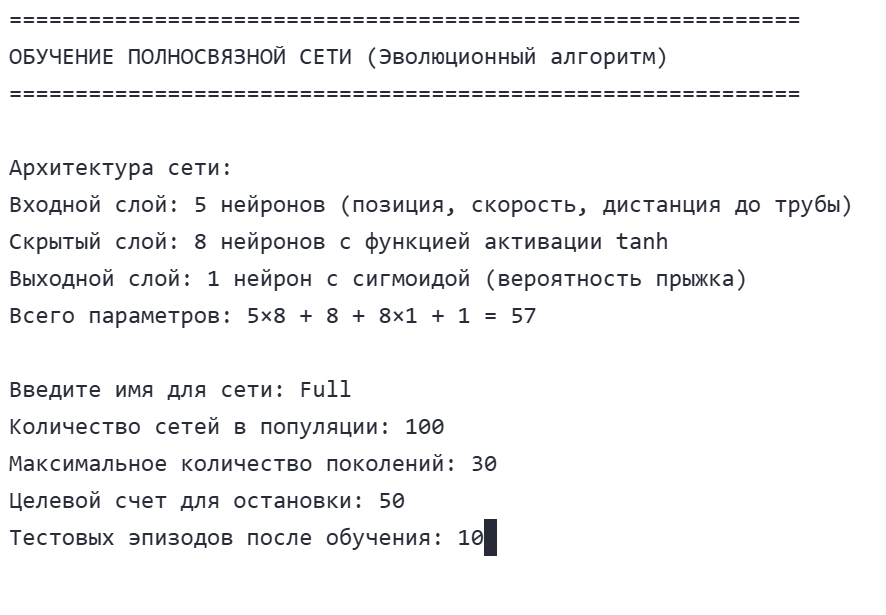
    println("FULLY CONNECTED NETWORK TRAINING (Evolutionary algorithm)")
    println("="^60)
    println("\Network architecture:")
    println("Input layer: 5 neurons (position, speed, distance to pipe)")
    println("Hidden layer: 8 neurons with TANH activation function")
    println("Output layer: 1 neuron with a sigmoid (jump probability)")
    println("Total parameters: 5×8 + 8 + 8×1 + 1 = 57")
    
    print("\Enter a name for the network: ")
    name = readline()
    
    print("Number of networks in the population: ")
    pop_size = parse(Int, readline())
    
    print("Maximum number of generations: ")
    max_generations = parse(Int, readline())
    
    print("Target account for the stop: ")
    target_score = parse(Float64, readline())
    
    print("Test episodes after training: ")
    test_episodes = parse(Int, readline())
    
    println("\The creation of a population...")
    population = [init_dense() for _ in 1:pop_size]
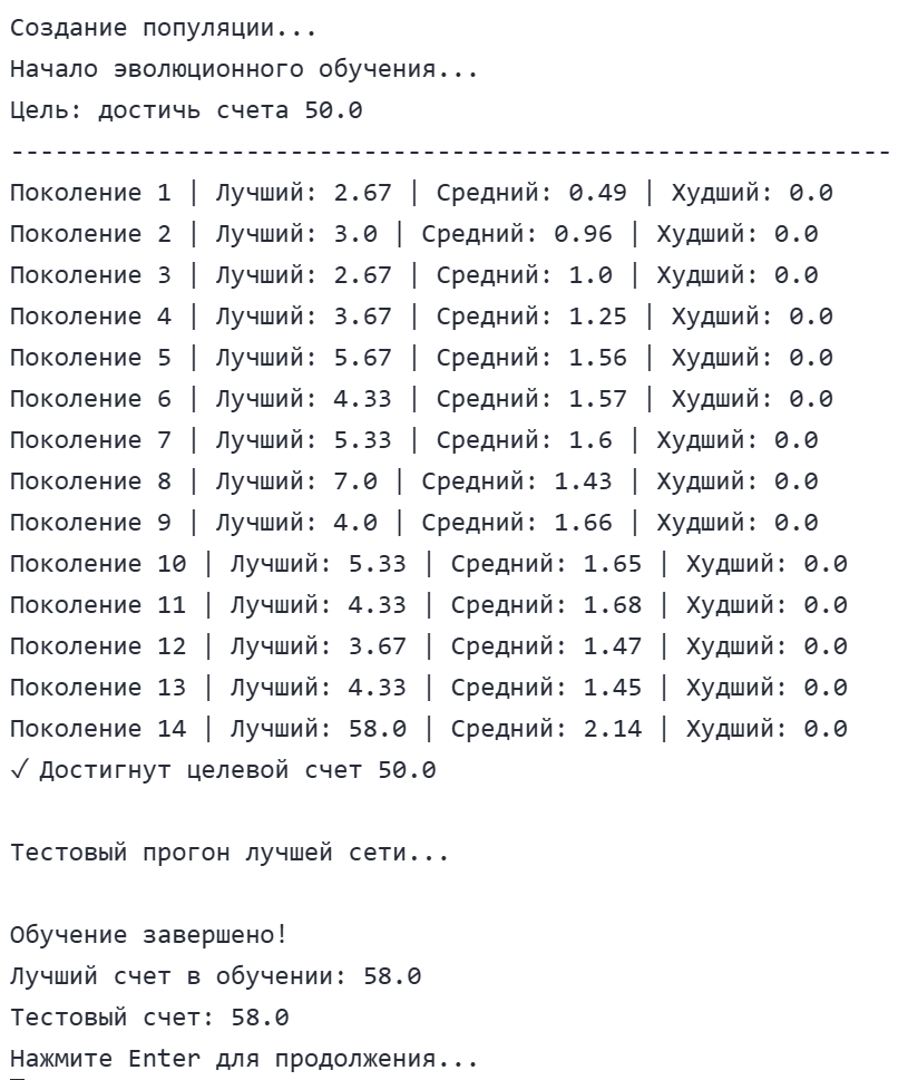
       println("The beginning of evolutionary learning...")
    println("Goal: Reach the $target_score account")
    println("-"^60)
    
    final_pop, training_stats, best_net, best_score = train_genetic!(
        population, :basic, 
        target_score=target_score, 
        max_generations=max_generations,
        mutation_rate=0.3
    )
    
    println("Test run of the best network...")
    test_score = evaluate_network(best_net, :basic, test_episodes)
    
    push!(results, NetworkResult(
        name,
        "Fully connected (5-8-1)",
        best_net,
        :basic,
        test_score,
        training_stats,
        57
    ))
    
    println("\The training is completed!")
    println("Best Learning score: ", round(best_score, digits=2))
    println("Test account: ", round(test_score, digits=2))
    println("Press Enter to continue...")
    readline()
    
    return results
end

function testing_menu(results)
    if isempty(results)
        println("There are no trained networks!")
        sleep(2)
        return
    end
    
    while true
        print("\033[2J\033[H")
        println("="^60)
        println("TEST RUN WITH GRAPHICS")
        println("="^60)
        println("\Select a network for testing (0 for exit):")
        
        for (i, r) in enumerate(results)
            println("$i. $(r.name) ($(r.architecture)): ", round(r.test_score, digits=2))
        end
        
        print("\nThe network number: ")
        input = readline()
        
        if input == "0"
            return
        end
        
        idx = tryparse(Int, input)
        if idx === nothing || idx < 1 || idx > length(results)
            println("Wrong number!")
            sleep(2)
            continue
        end
        
        chosen = results[idx]
        
        println("\Starting a network demo '$(chosen.name )'...")
        println("Press Ctrl+C to exit the demo")
        println("It starts in 3 seconds...")
        sleep(3)
        
        try
            score = run_episode(chosen.network, chosen.state_type; render=true, max_steps=1000)
            println("\The demonstration is over! Score: $score")
        catch e
            if !(e isa InterruptException)
                println("\Error during execution: $e")
            end
        end
        
        println("Press Enter to continue...")
        readline()
    end
end

function train_conv_menu(results)
    print("\033[2J\033[H")
    println("="^60)
    println("CONVOLUTIONAL NETWORK TRAINING (CNN) is an evolutionary algorithm")
    println("="^60)
    println("\Network architecture:")
    println("Entrance: 15×40 (height×width of the playing field)")
    println("Convolutional layer: 4 3×3 filters, ReLU activation")
    println("Fully connected layer: 1 neuron with a sigmoid")
    println("Total parameters: ~500")
    
    print("\Enter a name for the network: ")
    name = readline()
    
    print("Number of networks in the population: ")
    pop_size = parse(Int, readline())
    
    print("Maximum number of generations: ")
    max_generations = parse(Int, readline())
    
    print("Target account for the stop: ")
    target_score = parse(Float64, readline())
    
    print("Test episodes after training: ")
    test_episodes = parse(Int, readline())
    
    println("\The creation of a population...")
    population = [init_conv() for _ in 1:pop_size]
    
    println("The beginning of evolutionary learning...")
    println("Goal: Reach the $target_score account")
    println("-"^60)
        final_pop, training_stats, best_net, best_score = train_genetic!(
        population, :conv, 
        target_score=target_score, 
        max_generations=max_generations,
        mutation_rate=0.3
    )
    
    println("Test run of the best network...")
    test_score = evaluate_network(best_net, :conv, test_episodes)
    
    height, width = 15, 40
    filters = 4
    conv_params = 3 * 3 * 1 * filters + filters
    fc_params = (height-2) * (width-2) * filters + 1
    total_params = conv_params + fc_params
    
    push!(results, NetworkResult(
        name,
        "Convolutional (Conv3x3x4 → FC)",
        best_net,
        :conv,
        test_score,
        training_stats,
        total_params
    ))
    
    println("\The training is completed!")
    println("Best Learning score: ", round(best_score, digits=2))
    println("Test account: ", round(test_score, digits=2))
    println("Press Enter to continue...")
    readline()
    
    return results
end

function compare_results(results)
    if isempty(results)
        println("There are no results to compare!")
        sleep(2)
        return
    end
    
    print("\033[2J\033[H")
    println("="^60)
    println("COMPARISON OF TRAINED NETWORKS")
    println("="^60)
    
    sorted_results = sort(results, by=r->r.test_score, rev=true)
    
    println("\Network pricing (based on the test account):")
    println("-"^60)
    println("Place | Name | Architecture | Account | Parameters")
    println("-"^60)
    
    for (i, r) in enumerate(sorted_results)
        place = i == 1 ? "🥇" : i == 2 ? "🥈" : i == 3 ? "🥉" : "  $i."
        println("$place $(r.name) | $(r.architecture) | ", round(r.test_score, digits=2), " | $(r.params)")
    end
    
    if any(r -> !isempty(r.training_stats), sorted_results)
        println("\nStatistics of learning the best network:")
        best = sorted_results[1]
        if !isempty(best.training_stats)
            println("Number of generations: $(length(best.training_stats))")
            last_stat = best.training_stats[end]
            first_stat = best.training_stats[1]
            println("Initial average score: ", round(first_stat[3], digits=2))
            println("Final best score: ", round(last_stat[2], digits=2))
            println("Improvement: ", round(last_stat[2] - first_stat[2], digits=2))
        end
    end
    
    println("Press Enter to continue...")
    readline()
end

main_menu (generic function with 1 method)

To start the project, you need to call in the command line main_menu(). Below are the results of the launch of our project. For the exponent frequency, the parameters for both networks are set to be identical.

If you run the training of both types of neural networks yourself, you will notice that the convolutional network (CNN) is much slower to train than the fully connected one. This is due to a fundamental difference in the architecture and the amount of data being processed: CNN works with a complete 15x40 state matrix of the playing field (600 values), performing multiple convolution operations for several filters at each step. At the same time, a fully connected network receives only five preprocessed features as input, which requires orders of magnitude fewer calculations. This difference in learning rate clearly demonstrates the trade—off between model complexity and computational costs - more powerful architectures are able to solve problems better, but require significantly more resources for training.

Based on the presented results, several important conclusions can be drawn about the work of the evolutionary algorithm and the effectiveness of various neural network architectures in the Flappy Bird game task.

Both neural networks, Fully Connected and convolutional, achieved the same maximum score of 58.0 points.

The fully connected network has demonstrated exceptional efficiency: using only 57 parameters, it achieved the same result as the convolutional network with 2017 parameters (35 times more). This illustrates an important principle of machine learning: a more complex model does not always mean better performance, especially when the task can be successfully solved by simple means.

The evolutionary algorithm has shown high efficiency, achieving maximum results in just 14 generations. The initial average score of the population was only 0.49 points, which indicates that randomly initialized networks were practically unable to play. Over 14 generations, there has been an improvement of 57.51 points — an exponential increase in productivity, demonstrating the power of evolutionary optimization methods.

Below is provided how both networks decided to play as a result, both networks rise to the top of the field and calculate the moment when they need to stop jumping to get into the hole.

Conclusions

Simplicity versus complexity: For tasks with clear rules and limited state space, simple architectures can be just as efficient as complex ones, but require significantly less computing resources.
Evolutionary algorithms work: The gradient-free genetic approach has successfully optimized both architectures, showing its applicability to reinforcement learning tasks.
Algorithm convergence: Rapid convergence (14 generations) indicates well—chosen parameters of the evolutionary algorithm - population size, mutation rate, and selection strategy.
Performance ceiling: The same maximum score for both networks may indicate either the achievement of the maximum possible result in a given game configuration, or the limitations of the game environment itself.

These results confirm that a properly implemented evolutionary algorithm can effectively train neural networks even for complex tasks, and the choice of architecture should correspond to the specifics of the problem being solved, and not just strive for maximum complexity.