Simulation of automatic transmission operation
In this example, we will analyze the Chart tool and the logic of finite automata implemented by it, based on the principles of automatic gear shifting depending on speed.
At a simplified level, let's consider the differences in the operation of two types of algorithms – using states and using transition nodes.
At the beginning of the demonstration, we will declare an auxiliary function for running the model and proceed to the analysis of the implemented algorithms.
# Enabling the auxiliary model launch function.
function run_model( name_model)

    Path = (@__DIR__) * "/" * name_model * ".engee"

    if name_model in [m.name for m in engee.get_all_models()] # Checking the condition for loading a model into the kernel
        model = engee.open( name_model ) # Open the model
        model_output = engee.run( model, verbose=true ); # Launch the model
    else
        model = engee.load( Path, force=true ) # Upload a model
        model_output = engee.run( model, verbose=true ); # Launch the model
        engee.close( name_model, force=true ); # Close the model
    end
    sleep(5)
    return model_output
end
At the top level, the model contains two gearshift algorithms. The inputs for both charts are identical. The tables set the threshold values for the speed at which it is necessary to either increase or decrease the transmission, and the value of the current speed itself, set by the sine wave.
Next, let's look at each Chart individually. The upper block uses the logic of the nodes and, depending on the speed, outputs the gear shift parameter +-1, which allows you to increase or decrease the gear, which is stored in the loop. The initial transfer value in both cases is 1.
.png)
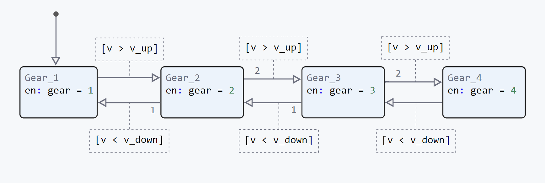
In the second case, depending on the speed, we switch between different states in which a suitable transmission is set for the input speed mode.
.png)
Now let's run the model itself and analyze the generated values.
run_model("car") # Launching the model.
We are reading the cached data from the simout.
In this case:
v is the speed of the car;
shift is the shift parameter for the gearbox algorithm implemented using nodes.;
gear_node – transmission values for Chart using nodes;
gear_state – transmission values for a Chart with states.
v = simout["car/Bias.1"];
v = collect(v);
shift = simout["car/ShiftChart.shift"];
shift = collect(shift);
gear_node = simout["car/gear"];
gear_node = collect(gear_node);
gear_state = simout["car/GearChart.gear"];
gear_state = collect(gear_state);
Now let's move on to analyzing the received data. Let's start with speed. As we can see from the graph below, the speed is set by a sine wave in the range from 0 to 120. The initial speed value is not zero. It is designed to visually demonstrate the differences between algorithms using nodes and states.
plot(v.time, v.value)
Next, we will analyze the system using nodes. As we can see, the initial value of this system in the first step is not the first gear, but the second. This is because the node immediately reported the increment of the counter.
plot(gear_node.time, gear_node.value)
plot!(shift.time, shift.value)
Now let's pay attention to the state-based system. The initial transfer value is 1. This is due to the fact that in the case of states in the absence of initialization logic, we will start with the input state and then go through a maximum of one state per clock cycle.
plot(gear_state.time, gear_state.value)
Now let's compare the values calculated by different transmission simulation systems. As we can see from the results below, the first two bars are different. This is due to the logic processing features described above.
difference = gear_state.value-gear_node.value;
print("The difference in gearshift logic: "*string(difference[1:3]))
Conclusion
In this demo, we analyzed the differences in the logic of nodes and states. Using this example, we got a clear idea of how different algorithms implemented using the Chart block are processed.