Pipeline pressure control using the Chart block
In this example, we will create a control logic for regulating the pipeline pressure. To create the algorithm, we will use the Chart block of the finite state machine library.
The principle of operation
A detailed description of the pipeline model is provided in the example along the following path:/user/start/examples/physmod/liquid_pressure_regulator. In this case, we will briefly describe the model and focus on the points necessary for management.
The structural diagram of the model is presented below, as well as in the model hydro_control_chart.engee.
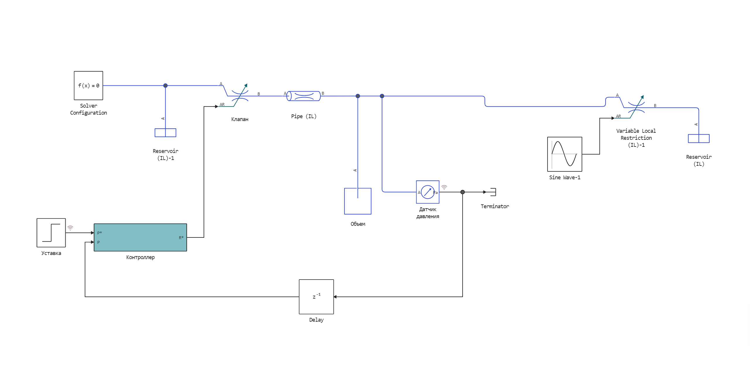
We need to maintain the pressure in the Volume unit. The pressure change is due to accidental leakage. For pressure measurement, a ** Pressure sensor** is present in the circuit. The pressure must be maintained according to the setpoint.
Control logic
To the entrance of the block The controller receives two signals: the setpoint and the value from the sensor. The signal from the output of the Controller is sent to the input of the Valve unit. This signal determines the cross-sectional area.
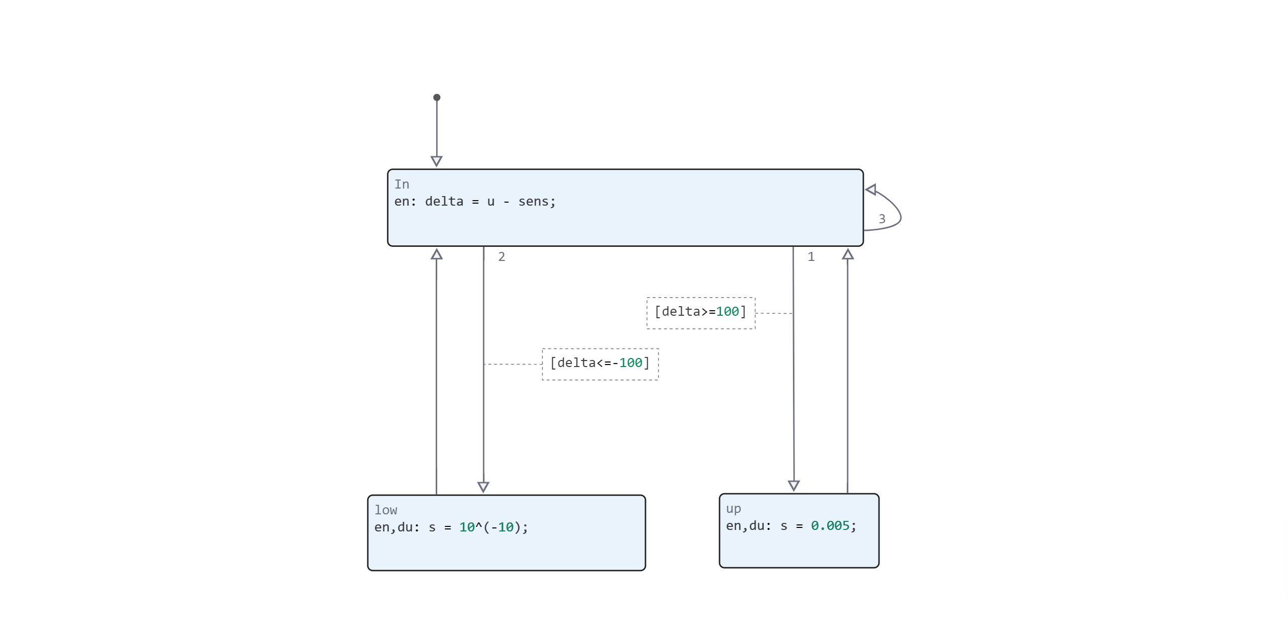
The Chart block from the Controller model contains three states. In the initial state, the difference between the set and measured pressure values is determined. Then there are three possible transitions.
- In the state of
lowif the difference is negative and exceeds the specified threshold. In this case, we minimize the cross-sectional area of the cathode hole.; - In the state of
upif the difference is positive and greater than the set threshold. We set the maximum cross-sectional area; - If the error is within the threshold value, we remain in the initial state.
Let's run the model and build graphs to evaluate the results.
Defining the function to load and run the model
Run the cell with the code to generate the model launch function.
function start_model_engee()
    try
        engee.close("hydro_control_chart", force=true) # closing the model
        catch err # if there is no model to close and engee.close() is not executed, it will be loaded after catch.
            m = engee.load("$(@__DIR__)/hydro_control_chart.engee") # loading the model
        end;

    try
        engee.run(m) # launching the model
        catch err # if the model is not loaded and engee.run() is not executed, the bottom two lines after catch will be executed.
            m = engee.load("$(@__DIR__)/hydro_control_chart.engee") # loading the model
            engee.run(m) # launching the model
        end
end
Getting simulation results
Let's run a simulation of the model using the function generated above.
try
    start_model_engee()
    catch err
    end;
Let's write the programmed signals into a variable simout. And we will convert them into an array of data.
result = simout;
res = collect(result)
We will write the values from the pressure sensor and the setpoint value to the variables.
control_signal = collect(res[1])
pressure = collect(res[2])
Visualization of the received data
using Plots
plot(control_signal[:,1], control_signal[:,2], label="Setpoint")
plot!(pressure[:,1], pressure[:,2], label="Pressure sensor")
At the 5th second of the simulation, the set pressure increased to 120 kPa. The pipeline pressure reached the setpoint at about 10 seconds and was in the area of the set threshold 100 Pa.
Conclusion
In this example, we have demonstrated pressure control in the pipeline using the control logic implemented in the Chart block.