gaspl
Attenuation of the RF signal due to absorption of gases by the atmosphere.
| Library |
|
Syntax
Function call
-
L = gaspl(R,F,T,p,den)— returns the attenuation of the signalLcaused by gas absorption in the atmosphere. Input argumentRsets the length of the signal path,F— the carrier frequency of the signal,T— ambient temperature,p— atmospheric pressure, andden— absolute humidity in the atmosphere.Function
gasplUses the atmospheric gas attenuation model of the International Telecommunication Union (ITU) [1] to calculate losses along the signal propagation path caused mainly by oxygen and water vapor. The model calculates attenuation as a function of ambient temperature, pressure, absolute humidity, and signal frequency.The function requires that the signal propagation path is completely located in a homogeneous medium — temperature
T, atmospheric pressurepand absolute humiditydenthe signal does not change along the propagation path. You can account for changes in atmospheric parameters with altitude using the functionstropoplandatmositu.The attenuation model is used only for frequencies in the range
1–1000GHz.
Arguments
Input arguments
# R is the length of the signal path, m
+
scalar | vector
Details
The length of the signal path in meters, used to calculate attenuation, given as a non-negative real scalar or length vector . You can specify multiple path lengths at the same time.
| Типы данных |
|
# F is the frequency of the signal, Hz
+
scalar | vector
Details
The frequency of the signal in Hz, specified as a positive real scalar or a non-negative real vector of length . You can specify multiple frequencies at the same time. The frequencies must be in the range 1–1000 GHz.
| Типы данных |
|
# T — ambient temperature, °C
+
scalar
Details
The ambient temperature in degrees Celsius, set as a real scalar.
| Типы данных |
|
# p — dry air pressure, Pa
+
scalar
Details
The pressure of dry air in Pa, set as a positive real scalar. One standard atmosphere at sea level is 101325 Pa.
| Типы данных |
|
# den — absolute humidity, g/m3
+
scalar
Details
The absolute humidity, or density of water vapor, in g/m 3, given as a non-negative real scalar. Maximum absolute humidity in the air at 30 °C is approximately 30.0 g/m3. Maximum absolute humidity in the air at 0 °C is approximately 5.0 g/m3.
| Типы данных |
|
Output arguments
# L — signal attenuation, dB
+
the matrix
Details
Signal attenuation in dB, returned as a real matrix of size on . Each row of the matrix represents a separate path, where — the number of paths. Each column represents a separate frequency, where — the number of frequencies.
Examples
Attenuation spectrum of atmospheric gas
Details
Calculate the attenuation spectrum in the range from 1 before 1000 GHz at atmospheric pressure 101.300 kPa and temperature 15 °C. Let’s construct a spectrum for the density of water vapor 7.5 g/m 3, and then the spectrum for dry air (zero density of water vapor).
Let’s set the attenuation frequencies.
F = (1:1000) * 1e9Assume that the length of the path is 1 km.
R = 1000.0Calculate the attenuation for air containing water vapor.
import EngeePhased.Functions: gaspl

T = 15
p = 101300.0
den = 7.5
L = gaspl(R, F, T, p, den)
Calculate the attenuation for dry air.
L0 = gaspl(R, F, T, p, 0.0)Let’s plot the attenuation graph.
plot(F / 1e9, [vec(L) vec(L0)],
     yscale = :log10,
      label = ["L" "L0"],
     xlabel = "Frequency (GHz)",
     ylabel = "Specific Attenuation (dB)")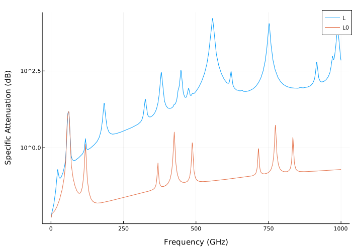
Plotting of attenuation due to atmospheric gases and free space
Details
First, we will plot the specific attenuation of atmospheric gases for frequencies from 1 GHz up to 1000 GHz. Assume that the pressure of dry air at sea level is 101.325 kPa, and the density of water vapor — 7.5 g/m3. Air temperature — 20 °C. Specific attenuation is defined as losses in dB/km. Then we will plot the actual attenuation at the frequency 10 GHz for the frequency range.
The construction of a graph of the specific attenuation of atmospheric gases
Let’s set the atmospheric temperature, pressure, and density of water vapor.
T = 20.0
p_atm = 101.325e3
rho_wv = 7.5
Let’s set the propagation distance, the speed of light, and the frequencies.
km = 1000.0
c = 299792458.0
freq = (1:1000) * 1e9
Let’s calculate and plot atmospheric gas losses.
import EngeePhased.Functions: gaspl

loss = gaspl(km, freq, T, p_atm, rho_wv)

plot(freq / 1e9, vec(loss),
     yscale = :log10,
     xlabel = "Frequency (GHz)",
     ylabel = "Specific Attenuation (dB/km)")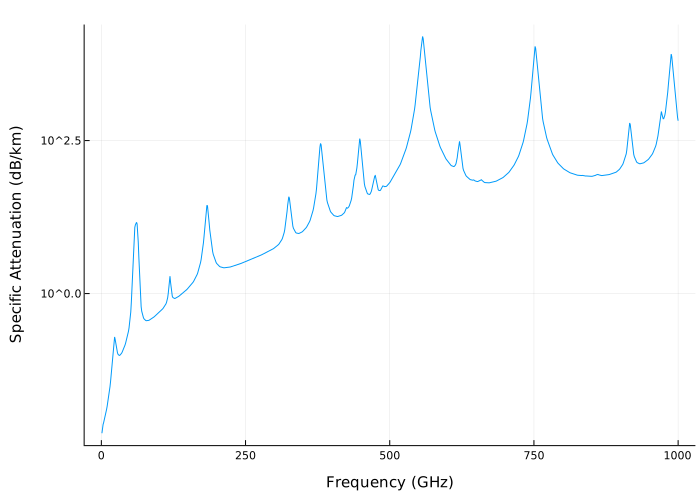
Plotting a graph of actual attenuation in the atmosphere and free space_
Calculate the losses in free space and losses in atmospheric gas at the frequency 10 GHz for ranges from 1 before 100 The frequency corresponds to the X-band radar station. Then we will plot the losses in free space and the total losses (atmosphere and free space).
import EngeePhased.Functions: fspl

ranges = (1:100) * 1000
freq_xband = 10e9
loss_gas = gaspl(ranges, freq_xband, T, p_atm, rho_wv)
lambda = c / freq_xband
loss_fsp = fspl(collect(ranges), lambda)

plot(ranges / 1e3, [vec(loss_gas + loss_fsp) vec(loss_fsp)],
     xscale = :log10,
      label = ["Atmospheric + Free Space Loss" "Free Space Loss"],
     xlabel = "Range (km)",
     ylabel = "Loss (dB)",
     legend = :bottomright)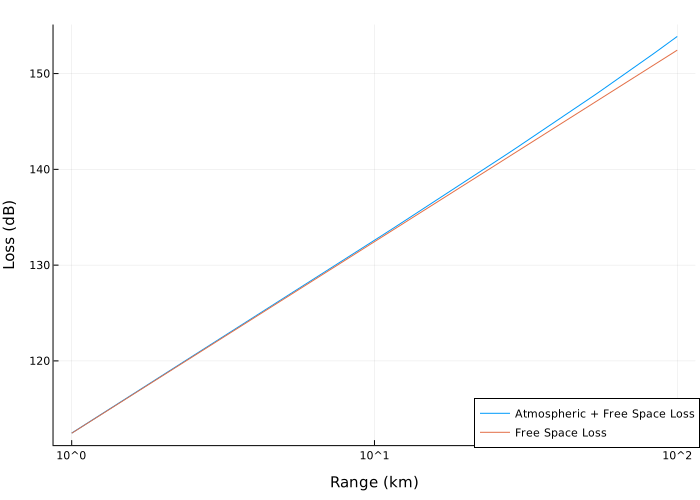
Additional Info
Attenuation model in atmospheric gases
Details
This model calculates the attenuation of signals propagating through atmospheric gases.
Electromagnetic signals are attenuated as they propagate through the atmosphere. This effect is mainly due to the resonant absorption lines of oxygen and water vapor, with nitrogen contributing less. The model also includes a continuous absorption spectrum below 10 GHz. The ITU atmospheric gas attenuation model [1] is used. The model calculates the specific attenuation (attenuation per kilometer) as a function of temperature, pressure, absolute humidity, and signal frequency. The atmospheric gas model is valid for frequencies from 1 before 1000 GHz and is applicable to polarized and unpolarized fields.
The formula for the specific attenuation at each frequency:
Value It represents the imaginary part of the complex atmospheric refraction and consists of a spectral line component and a continuous component.:
The spectral component is the sum of discrete spectral terms consisting of a localized function of the frequency band multiplied by the intensity of the spectral line . For atmospheric oxygen, the intensity of each spectral line is
where — ambient temperature in kelvin, — dry air pressure in gPa.
For atmospheric water vapor, the intensity of each spectral line is
where — partial pressure of water vapor in gPa. It is related to the density of water vapor. the ratio
The total atmospheric pressure is .
For each oxygen line depends on two parameters: and . Similarly, each water vapor line depends on two parameters: and . The ITU documentation, listed in the Literature section, contains tables of these parameters as functions of frequency.
Localized frequency band functions They are complex frequency functions described in [1]. These functions depend on the parameters of the empirical model, which are also given in the table [1].
This model is applicable to both narrowband and broadband atmospheric attenuation. To calculate the total attenuation for narrowband signals along the path, the function multiplies the specific attenuation by the path length. . Then the total attenuation is . To apply the attenuation model to broadband signals, first divide the broadband signal into frequency sub-bands and apply attenuation to each sub-band. Then sum up all the attenuated subband signals into a total attenuated signal.