periodogram
Estimation of the spectral power density by the periodogram method.
| Library |
|
Syntax
Function call
-
pxx,f,pxxc = periodogram(_,Name=Value,out=:data)— sets additional parameters using arguments like «name-value» for any of the previous syntax options. The function also returns the bounds of the confidence interval.pxxcif a level is specified for estimating the spectral power densityConfidenceLevel=p.
-
periodogram(_)— plots the estimation of the SPM or power spectrum. For this syntax, you can additionally pass parameters for displaying the final graph. For example, if you callperiodogram(x, color = :red), then the graph will be red. If an argument is specifiedConfidenceLevel, then for each column, the confidence intervals will also be shown as dotted lines.
Arguments
Input arguments
# x — input signal
+
vector | the matrix
Details
An input signal specified as a vector or matrix. If x — matrix, function periodogram considers its columns as independent channels.
| Типы данных |
|
| Support for complex numbers |
Yes |
# win — window
+
fill(1, size(x, 1)) (default) | a real or complex vector
Details
A window defined as a vector of the same length as the input signal. If the argument is win not specified, function periodogram uses a rectangular window.
A standard rectangular window is characterized by a side lobe suppression level equal to 13.3 dB; this can lead to masking of spectral components, the level of which is lower than this value (relative to the peak value of the spectrum). Choosing other types of windows allows you to find a compromise between the resolution (for example, when using a rectangular window) and the degree of suppression of the side lobes (for example, when using a Hannah window).
|
| Типы данных |
|
# nfft is the number of points in the DFT
+
max(256, nextpow(2, size(x, 1))) (by default) | a positive integer
Details
The number of points in the DFT, given as a positive integer scalar.
If the argument is nfft if not specified, the function uses the value , where . Symbols denote rounding up, and length(win).
| Типы данных |
|
# freq — normalized or cyclic frequencies
+
the real vector
Input arguments «name-value»
Specify optional argument pairs as Name=Value, where Name — the name of the argument, and Value — the appropriate value. Type arguments «name-value» they should be placed after the other arguments, but the order of the pairs does not matter. You can specify multiple pairs «name-value».
#
fs — sampling
rate
NaN (by default) | positive scalar
Details
The sampling rate, set as a positive scalar. The sampling rate is the number of samples per unit of time. If the unit of time is seconds, then the sampling frequency is expressed in Hz.
# freqrange — frequency range of SPM assessment
+
"onesided" | "twosided"
Details
The frequency range for the SPM assessment, set as "onesided" or "twosided".
For signals with real values, the default value is "onesided". For complex signals, the default value is "twosided", and specifying the value "onesided" leads to an error.
-
Meaning
"onesided"— returns a one-way periodogram of the real input signal.-
If the value of the argument is
nffteven, then the argumentpxxhasnfft/2 + 1rows and is calculated on the interval[0, π]radians to count. -
If the value of the argument is
nfftIf it’s an odd number, thenpxxhas(nfft + 1)/2rows and is calculated on the interval[0, π)radians to count. If you specifyfs, then the intervals will be respectively[0, fs/2]cycles per unit of time and[0, fs/2)cycles per unit of time.
-
-
Meaning
"twosided"— returns a two-way periodogram of a real or complex signal. Argumentpxxhasnfftrows and is calculated on the interval[0, 2π)radians to count. If you specify an argumentfs, then the interval will be[0, fs)cycles per unit of time.
# centered — is the frequency range centered
+
false (by default) | true
Details
Enabling the centering of the frequency range, set as false or true.
# spectrumtype — scaling of the power spectrum
+
"psd" (default) | "power"
Details
Scaling of the power spectrum, set to one of the following values:
-
"psd"— functionperiodogramreturns the spectral power density; -
"power"— the function scales each SPM estimate by the equivalent noise frequency band of the window and returns an estimate of the power at each frequency.
The table shows the scaling ratio between the SPM estimate and the estimate of the power spectrum returned to pxx, with the specified input signal x, the window vector win, the number of points in the DFT nfft and the sampling rate fs.
| Sampling rate | The scaling ratio |
|---|---|
|
Then |
|
Then |
# ConfidenceLevel — confidence interval for the assessment of SPM
+
NaN (by default) | a real number in the range from 0 to 1
Details
The coverage probability for the SPM estimate, given as a scalar in the range (0, 1).
If specified ConfidenceLevel = p,
function periodogram returns in the output argument pxxc the lower and upper bounds of the confidence interval with the level p × 100% for true SPM.
# out — type of output data
+
:plot (by default) | :data
Details
Type of output data:
-
:plot— the function returns a graph; -
:data— the function returns data.
Output arguments
# pxx — estimation of SPM or power spectrum
+
vector | the matrix
Details
The estimate of the SPM or power spectrum returned as a real non-negative column vector or matrix.
-
Each column
pxxIt represents an estimate of the SPM or the power spectrum of the corresponding column.xdepending on how the argument is setspectrumtype. -
The measurement units of the SPM estimate are the squares of the input signal value per unit frequency. For example, if the input data is
xset in volts, sampling ratefs— in hertz, and the resistance is1Ohms, then the SPM estimate will be expressed in Watts/Hz. -
The units of measurement of the power spectrum are the squares of the input signal. For example, if the input data is
xThey are set in volts, and the resistance is1Ohms, then the estimate of the power spectrum will be expressed in watts.
# f — frequencies associated with the assessment of SPM
+
vector
# pxxc — confidence intervals
+
the matrix
Details
The bounds of the confidence intervals returned as a real matrix.
-
The matrix
pxxchas as many rows aspxx. -
The matrix
pxxcit has twice as many columns aspxx.-
The odd columns contain the lower bounds of the confidence intervals.
-
The even columns contain the upper bounds of the confidence intervals.
Thus,
pxxc[m, 2 * n − 1]— this is the lower limit of the confidence interval, andpxxc[m, 2 * n]— the upper limit of the confidence interval corresponding to the estimatepxx[m, n]. -
-
The probability of covering confidence intervals is determined by the value of the argument
ConfidenceLevel.
Dependencies
To use this argument, specify the value for the argument ConfidenceLevel.
| Типы данных |
|
Examples
A periodogram with standard parameters
Details
We obtain a periodogram of the input signal, which is a discrete sinusoid with an angular frequency rad/count, to which white noise is added with a distribution .
Let’s form the input signal. The length of the signal is 320 counts. Let’s calculate the periodogram using the rectangular window and the default DFT length. The length of the DFT is chosen equal to the nearest power of two exceeding the length of the signal, that is 512 points. Since the signal is real and has an even length, the periodogram is one-sided and contains 512/2 + 1 a period.
import EngeePhased.Functions: periodogram

n = collect(0:319);
x = cos.(pi ./ 4 .* n) .+ randn(size(n));
periodogram(x)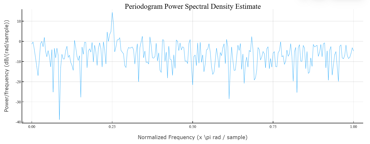
Modified periodogram with a Hamming window
Details
We obtain a modified periodogram of the input signal, which is a discrete sinusoid with an angular frequency rad/count, to which white noise is added with a distribution .
Let’s form the input signal. The length of the signal is 320 counts. Let’s calculate the periodogram using the rectangular window and the default DFT length. Let’s calculate the modified periodogram using the Hamming window and the default DFT length. The length of the DFT is chosen equal to the nearest power of two exceeding the length of the signal, that is 512 points. Since the signal is real and has an even length, the periodogram is one-sided and contains 512/2 + 1 a period.
import EngeePhased.Functions: periodogram
import EngeeDSP.Functions: hamming

n = collect(0:319)
x = cos.(pi ./ 4 .* n) .+ randn(size(n));
periodogram(x,hamming(length(x)))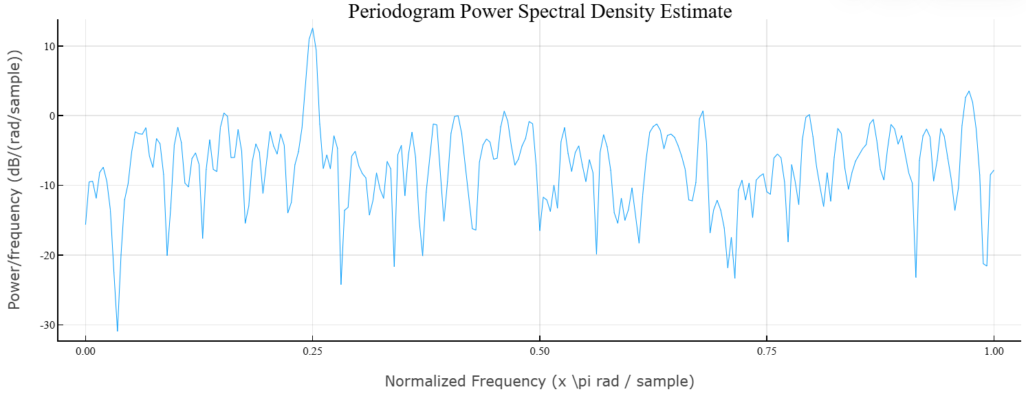
The length of the DFT is the same as the length of the signal
Details
We obtain a periodogram of the input signal, which is a discrete sinusoid with an angular frequency rad/count, to which white noise is added with a distribution . We use a DFT length equal to the length of the signal.
Let’s form the input signal. The length of the signal is 320 counts. Let’s calculate the periodogram using a rectangular window (by default) and a DFT length equal to the length of the signal. Since the signal is real, a one-way periodogram of length is returned by default. 320/2 + 1.
import EngeePhased.Functions: periodogram

n = collect(0:319);
x = cos.(pi ./4 .* n) .+ randn(size(n));
nfft = length(x);
periodogram(x,nfft=nfft)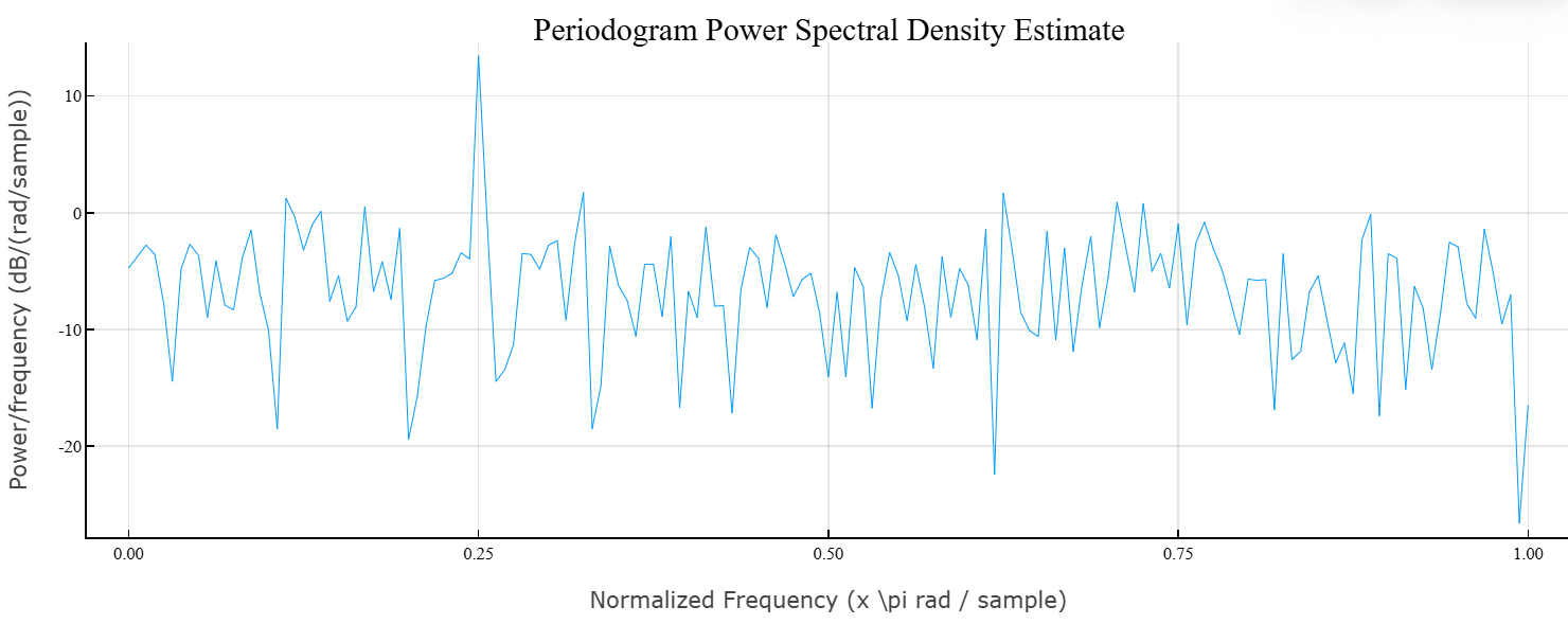
A periodogram based on a set of normalized frequencies
Details
We obtain a periodogram of the input signal consisting of two discrete sinusoids with angular frequencies and rad/counting on the background of additive white noise with distribution . We obtain two-sided estimates of the periodogram at frequencies and rad/countdown.
import EngeePhased.Functions: periodogram

n = collect(0:319);
x = cos.(pi ./ 4 .* n) .+ 0.5 .* sin.(pi ./ 2 .* n) .+ randn(size(n));

pxx,w = periodogram(x,freq=[pi/4, pi/2],out=:data)
pxx
2×1 Matrix{Float64}:
10.087037418886014
1.7539619680699419Let’s compare the result with a one-sided periodogram. The values of the two-sided periodogram are half of the values of the one-sided periodogram. When calculating a periodogram for a specific set of frequencies, the result is a two-way estimate.
pxx1,w1 = periodogram(x,out=:data)

plot(w1 ./ π, pxx1; label="pxx1")
plot!(w ./ π, 2 .* pxx; label="2*pxx", seriestype=:scatter)
xlabel!("Normalized Frequency (× π rad/sample)")
title!("Periodogram Power Spectral Density Estimate")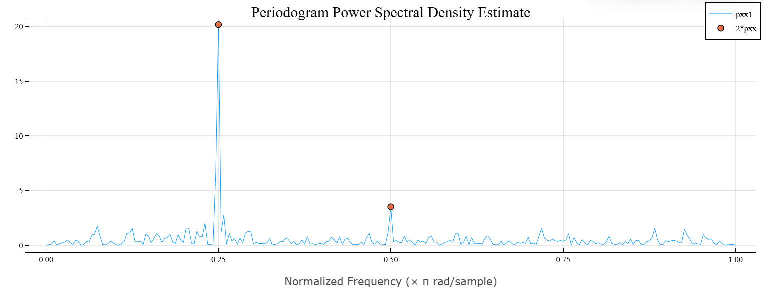
A periodogram based on a set of cyclic frequencies
Details
Let’s form a signal consisting of two sinusoids with frequencies 100 and 200 Hz on the background of additive white noise with distribution . The sampling rate is 1 kHz. Let’s calculate a two-way periodogram for frequencies 100 and 200 Hz.
import EngeePhased.Functions: periodogram

fs = 1000;
t = collect(0:0.001:1-0.001);
x = cos.(2 .* pi .* 100 .* t) .+ sin.(2 .* pi .* 200 .* t) .+ randn(size(t));

freq = [100, 200];
pxx,w = periodogram(x,freq=freq,fs=fs, out=:data)
pxx
2×1 Matrix{Float64}:
0.28289790057149083
0.26824883574824315Centered periodogram
Details
We get a periodogram of a sinusoidal signal with a frequency 100 Hz on the background of additive white noise with distribution . The sampling rate is 1 kHz. We use the centering option to get a periodogram centered relative to the zero frequency.
import EngeePhased.Functions: periodogram

fs = 1000;
t = collect(0:0.001:1-0.001);
x = cos.(2 .* pi .* 100 .* t) .+ randn(size(t));
periodogram(x,nfft=length(x), fs=fs, freqrange="onesided", centered=true)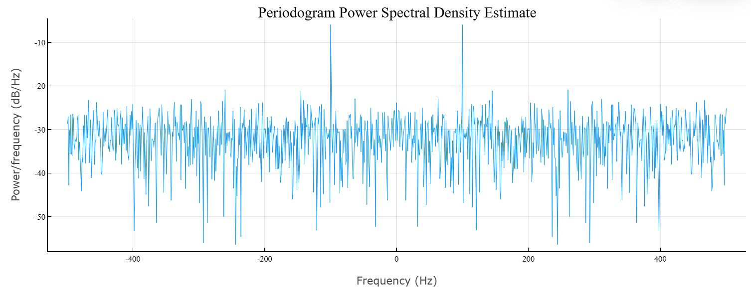
95 confidence intervals%
Details
Let’s form a signal consisting of two sinusoids with frequencies 100 and 150 Hz on the background of additive white noise with distribution . The amplitude of both sinusoidal signals is 1. The sampling rate is 1 kHz. We will get an estimate of the SPM using the periodogram method with `95`with % confidence intervals.
import EngeePhased.Functions: periodogram

fs = 1000;
t = collect(0:1/fs:1-1/fs);
x = cos.(2 .* pi .* 100 .* t) .+ sin.(2 .* pi .* 150 .* t) + randn(size(t));
periodogram(x, nfft=length(x), fs=fs, ConfidenceLevel = 0.95)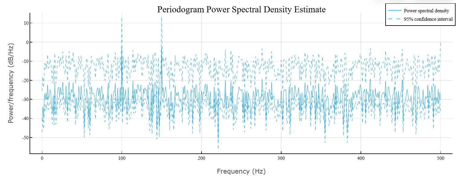
Estimation of sinusoid power
Details
Let’s estimate the power of the sinusoidal signal at a given frequency using the option "power".
Let’s form a sinusoidal signal with a frequency 100 Hz and duration 1 one second at the sampling rate 1 kHz. The amplitude of the sine wave is 1.8, which corresponds to the power 1.82/2 = 1.62.
import EngeePhased.Functions: periodogram
import EngeeDSP.Functions: hamming

fs = 1000;
t = collect(0:1/fs:1-1/fs);
x = 1.8 .* cos.(2 .* pi .* 100 .* t);
pxx,f = periodogram(x, hamming(length(x)), length(x), fs=fs, spectrumtype="power", out = :data);
idx = argmax(pxx)
pwrest = pxx[idx]
println("The maximum power occurs at $(f[idx]) Hz")
println("The power estimate is $pwrest")
The maximum power occurs at 100.0 Hz
The power estimate is 1.6200000517531614Additional Info
Periodogram
Details
The periodogram is a nonparametric estimate of the power spectral density (SPM) of a stationary, broadly random process. A periodogram is a Fourier transform of a biased estimate of an autocorrelation sequence. For the signal , sampled with frequency fs counts per unit of time, the periodogram is defined as follows:
where — sampling interval. In the case of a one-sided periodogram, the values are at all frequencies except 0 and Nyquist frequencies , multiplied by 2 to save overall power.
If the frequencies are expressed in radians per count, the periodogram is defined as
The frequency range in the above equations may vary depending on the value of the argument. freqrange.
The integral of the true SPM for one period (equal to for cyclic frequency and for a normalized frequency) is equal to the variance of a stationary, broadly random process:
For normalized frequencies, the integration limits should be adjusted accordingly.
Modified periodogram
Details
When calculating the modified periodogram, the input time series is multiplied by the window function. A suitable window function is non-negative and decreases to zero at the start and end points. Multiplying a time series by a window function ensures a smooth rise and fall of data values, which helps to reduce the spreading effect in the periodogram.
If is a window function, then the modified periodogram is defined as follows:
where — sampling interval.
If the frequencies are expressed in radians per count, the modified periodogram is defined as
The frequency range in the above equations may vary depending on the value of the argument. freqrange.
Literature
-
Auger, François, and Patrick Flandrin. Improving the Readability of Time-Frequency and Time-Scale Representations by the Reassignment Method. IEEE® Transactions on Signal Processing. Vol. 43, May 1995, pp. 1068–1089.
-
Fulop, Sean A., and Kelly Fitz. Algorithms for computing the time-corrected instantaneous frequency (reassigned) spectrogram, with applications. Journal of the Acoustical Society of America. Vol. 119, January 2006, pp. 360–371.