Simulation of GPS sensor noise
This example shows how to use the GPS unit to simulate the noise that the GNSS sensor adds to the position and velocity inputs.
Description of the model
This model defines the trajectory by generating values for the X, Y, and Z coordinates (both position and velocity) as separate sinusoidal signals and combines them using Mux blocks.
Since the GNSS (GPS) unit requires discrete signals, the position and velocity vectors pass through the Rate Transition blocks and only then enter the inputs of the Position and Velocity ports of the GPS unit. All parameters of the GPS unit are left unchanged except for the Vertical position accuracy parameter, which is set to 1.5 m to match the trajectory scale.
Let's open this model:
cd(@__DIR__) # Go to the folder with the example
engee.open("simulate-gps-sensor-noise.engee");
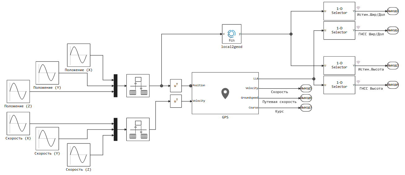
The model has an Engee Function block, which implements a code for converting the parameters of the true position from a topocentric coordinate system to a geodetic one.
Let's launch the model:
data = engee.run("simulate-gps-sensor-noise");
And let's compare the output signals of the GPS unit with the true values of the signals.
plot(
    plot( data["The truths.Shir/Dol"].time,
        [first.(data["The truths.Shir/Dol"].value) last.(data["The truths.Shir/Dol"].value) first.(data["GNSS Shir/Dol"].value) last.(data["GNSS Shir/Dol"].value)],
        lw=2, titlefont=font(11), guidesfont=font(8),
        xlabel="Time, from", ylabel="Degrees", title="Latitude and Longitude (True and GNSS)"),
    plot( data["The truths.Height"].time, [data["The truths.Height"].value first.(data["GNSS Height"].value)],
        lw=2, titlefont=font(11), guidesfont=font(8),
        xlabel="Time, from", ylabel="Height, m", title="Altitude (True and GNSS)" ),
    layout=(1,2), size=(900,400), leg=false
)
We will also study speed measurements.:
plot(
    plot(data["Course"].time, first.(data["Course"].value), title="GPS course", lw=2, titlefont=font(11), guidesfont=font(8), xlabel="Time, from", ylabel="Degrees"),
    plot(data["Speed"].time, [reduce(vcat, data["Speed"].value) reduce(vcat, data["The truths.Speed"].value)], title="Speed (true and according to GNSS)", lw=2, titlefont=font(11), guidesfont=font(8), xlabel="Time, from", ylabel="Meters per second"),
    plot(data["Ground speed"].time, first.(data["Ground speed"].value), title="Ground speed according to GNSS", lw=2, titlefont=font(11), guidesfont=font(8), xlabel="Time, from", ylabel="Meters per second"),
    layout=(1,3), size=(900,300), leg=false
)
Conclusion
We checked the operation of the GPS unit and made sure that it was possible to add complex error models to the model and calculate noisy trajectory indicators.