We are modeling the first artificial satellite of the Earth

In this project, we will build the ground track of the PS-1 satellite, launched on October 4, 1957.

Preparation and launch

Let's get ready for work: open the coast contour map and set the desired projection for it.

Pkg.add(["SatelliteToolbox", "Shapefile", "Proj"])

We downloaded the map from the [Natural Earth] repository in advance (https://www.naturalearthdata.com /). You will find more extensive information for working with maps here.

using Shapefile, Downloads, Proj

shp_path = joinpath(@__DIR__, "map", "ne_110m_coastline.shp");
table = Shapefile.Table(shp_path);

trans = Proj.Transformation("+proj=longlat", "+proj=robin +lon_0=0 +x_0=0 +y_0=0");

Now let's run the model. We will get several state vectors.

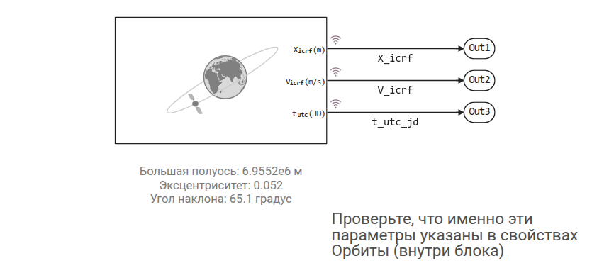
engee.open("sputnik_model.engee") # Please comment if the model is already open.
data = engee.run("sputnik_model")

X_icrf = collect(data["X_icrf"]).value;
V_icrf = collect(data["V_icrf"]).value;
t_utc_jd = collect(data["t_utc_jd"]).value;

df = DataFrame( time = data["X_icrf"].time, t_utc_jd = t_utc_jd, X_icrf = X_icrf, V_icrf = V_icrf);

We have assembled the vectors into a DataFrame object, now we will fill it with additional parameters.

Translating coordinates to other systems

To display graphs, it is usually interesting to translate coordinates into a geocentric and geodetic system. Consider the following considerations:

for our project, the ICRF system is almost identical to the GCRF (ECI) system, with errors of the order of one meter
the observer will be located in Moscow
topocentric coordinates are plotted using the WGS84 ellipsoid

using DataFrames
using SatelliteToolbox
using LinearAlgebra

# Where is the observer located
OBS_LLA = [deg2rad(55.7558), deg2rad(37.6173), 0.2e3]
eop = fetch_iers_eop()

# Adding new columns
df[!, :lon] = zeros(length(df[!, :time]))
df[!, :lat] = zeros(length(df[!, :time])) 
df[!, :alt] = zeros(length(df[!, :time]))
df[!, :az] = zeros(length(df[!, :time]))
df[!, :el] = zeros(length(df[!, :time]))
df[!, :range] = zeros(length(df[!, :time]))

# The parameters of the Earth for converting the coordinates of the observer
a = 6378137.0
lat_obs, lon_obs, alt_obs = OBS_LLA
x_obs = (a + alt_obs) * cos(lat_obs) * cos(lon_obs)
y_obs = (a + alt_obs) * cos(lat_obs) * sin(lon_obs)
z_obs = (a + alt_obs) * sin(lat_obs)

for i in 1:length(df[!, :time])
    # ICRF → ITRF conversion
    sv_icrf = OrbitStateVector(df[i, :t_utc_jd], df[i, :X_icrf], df[i, :V_icrf])
    sv_ecef = sv_eci_to_ecef(sv_icrf, GCRF(), ITRF(), df[i, :t_utc_jd], eop)
    
    # Geodetic coordinates
    lat, lon, alt = ecef_to_geodetic(sv_ecef.r)
    df[i, :lon] = rad2deg(lon)
    df[i, :lat] = rad2deg(lat)
    df[i, :alt] = alt
    
    # Topocentric coordinates
    Δr = sv_ecef.r - [x_obs, y_obs, z_obs]
    range_val = norm(Δr)
    
    # ENU coordinates (Local coordinate system of the observer east-north-top)
    e = -sin(lon_obs)*Δr[1] + cos(lon_obs)*Δr[2]
    n = -sin(lat_obs)*cos(lon_obs)*Δr[1] - sin(lat_obs)*sin(lon_obs)*Δr[2] + cos(lat_obs)*Δr[3]
    u = cos(lat_obs)*cos(lon_obs)*Δr[1] + cos(lat_obs)*sin(lon_obs)*Δr[2] + sin(lat_obs)*Δr[3]
    
    az = atan(e, n) % (2π)
    el = atan(u, sqrt(e^2 + n^2))
    
    df[i, :az] = rad2deg(az)
    df[i, :el] = rad2deg(el)
    df[i, :range] = range_val
end

Graph of the Earth's trajectory of the spacecraft

The obtained geodetic coordinates can simply be plotted, but in order for them to be plotted as lines, you first need to divide each circle around the planet into separate segments so as not to observe unnecessary jumps on the graph (between longitude 180 and -180).

ground_track_df = select(df, [:lon, :lat, :time])

# The ground route of the orbit
ground_track_lons = df.lon
ground_track_lats = df.lat

# We divide it into segments
jumps = findall(i -> abs(ground_track_lons[i+1] - ground_track_lons[i]) > 180, 1:length(ground_track_lons)-1)
segments = []
start_idx = 1

for jump_idx in jumps
    push!(segments, (ground_track_lons[start_idx:jump_idx], ground_track_lats[start_idx:jump_idx]))
    start_idx = jump_idx + 1
end

# Adding the last segment
push!(segments, (ground_track_lons[start_idx:end], ground_track_lats[start_idx:end]))

# We draw each segment separately
plot(title="The ground route of the orbit")
for (seg_lons, seg_lats) in segments
    xy_transf = trans.(seg_lons, seg_lats)
    xx,yy = getindex.(xy_transf, 1), getindex.(xy_transf, 2)
    plot!(xx, yy, legend=false, linecolor=:blue)
end
plot!()

for shape in table
    x = [point.x for point in shape.geometry.points]
    y = [point.y for point in shape.geometry.points]
    xy_transf = trans.(x, y)
    xx,yy = getindex.(xy_transf, 1), getindex.(xy_transf, 2)
    plot!(xx, yy, c=1, lw=0.5, fill=:lightblue)
end
plot!()

Graph of satellite observability from the Earth's surface

To plot the satellite's observability from the point where the observer is located, we calculated the topocentric azimuth and declination. We will separate only those segments of the trajectory when the satellite was above the horizon.

# Points above the horizon
skyplot_mask = df.el .> 0

skyplot_az = df.az # df.az[skyplot_mask] # This data can already be deduced
skyplot_el = df.el # df.el[skyplot_mask] # but let's divide them into segments

true_indices = findall(skyplot_mask)    # We divide it into continuous segments
gaps = findall(diff(true_indices) .> 1) # We find gaps in the indexes
boundaries = vcat([1], gaps .+ 1, [length(true_indices) + 1]) # Segment boundaries

segments_az = Vector{Vector{eltype(skyplot_az)}}()
segments_el = Vector{Vector{eltype(skyplot_el)}}()
for i in 1:length(boundaries)-1
    start_idx = boundaries[i]
    end_idx = boundaries[i+1] - 1
    segment_indices = true_indices[start_idx:end_idx]
    push!(segments_az, skyplot_az[segment_indices])
    push!(segments_el, skyplot_el[segment_indices])
end

In a separate cell, we will display a hemisphere and plot all the segments on it in order to see the trajectory of the satellite as it was seen from the surface of the Earth.

# Creating a hemisphere
n = 30
u = range(0, 2π; length=n)
v = range(0, π/2; length=n)
x_sphere = cos.(u) .* sin.(v)'
y_sphere = sin.(u) .* sin.(v)'
z_sphere = ones(n) .* cos.(v)'

# We draw a hemisphere
surface(x_sphere, y_sphere, z_sphere, alpha=0.4, legend=false)
xlabel!("East"); ylabel!("North"); zlabel!("Top")

# Drawing trajectory segments
for (azimuths,elevations) in zip(segments_az, segments_el)
    # Convert to Cartesian coordinates
    az_rad = deg2rad.(azimuths)
    el_rad = deg2rad.(elevations)
    x = cos.(el_rad) .* cos.(az_rad)
    y = cos.(el_rad) .* sin.(az_rad)
    z = sin.(el_rad)

    plot!(x, y, z, lw=4)
end
plot!(legend=false, title="Satellite visibility chart (Moscow)")

We can see when and how the satellite was observed from a point in Moscow. And since the satellite's state vector also includes velocity, we can calculate the Doppler shift and specify exactly how its signal sounded, calling us to new achievements.

Conclusion

We obtained the coordinates of the PS-1 satellite during 60,000 seconds of observation (the real satellite spent about 8 million seconds in orbit) and built a couple of useful graphs to interpret the trajectory of this spacecraft.