Simulation of battery operation modes based on finite automata

Library "Finite automata" is a tool designed for convenient graphical representation of system states and description of the logic of transitions between them when certain conditions are met. The finite state machine-based approach increases the visibility, reliability, and scalability of complex control logic algorithms.

In this example, we will take a step-by-step look at the basic concepts of the Finite Automata library and simulate the operating modes of a simple battery.

Step 1. State Machines

Let's add the [Chart] block to the canvas(https://engee.com/helpcenter/stable/en/state-machines/chart.html ), let's go into it and create two states:

The battery can be connected to an external power source and charged (condition Charge).
Otherwise, it is discharged (state Discharge).

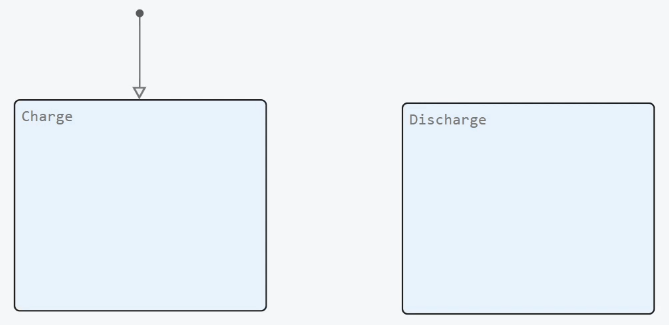
We have just begun to develop the simplest state machine. State machines are designed to simulate systems that can be in one of the predefined states or modes of operation.

Let's add transitions between the states, and also pay attention to the fact that Charge the default transition is enabled. It is indicated by a dot at the end and indicates the state that will be active at the first step of the simulation.

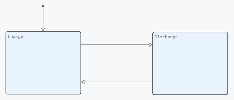
The other two transitions are still unconditional. This means that if we run a simulation, a transition from one state to another will be performed at each step. That is, they will become active in turn.

Let's write down the transition conditions - logical expressions, if true, the transitions will be considered valid. They should be indicated in square brackets.:

If the battery is charging and the variable isCharging takes the value false, the transition to the state is in progress Discharge.
And vice versa, if the battery is low and the variable isCharging takes the value true, the transition to the state is in progress Charge.

By the way, in addition to the condition, we could specify the action that should be performed during the transition. It is written in curly brackets and is most often used to assign variables.

Let's consider the algorithm for executing a state machine in more detail.:

In the first step of the simulation, the state machines start executing from the default transition.
Subsequent calls to the Chart block result in execution from the last active state.
After that, the conditions of transitions originating from this state begin to be checked. If the condition is valid (that is, it takes the value "True"), then the actions are performed and the transition is carried out.
Otherwise, other transitions are being tested. If they are missing, or none of the transitions are valid, the current state remains active.

Now let's write the code inside the states.:

Let the battery not produce power during charging, but when discharging, it produces a load of 3.5 watts. We will assign these values only when entering the state, so we will write a keyword in front of them. entry.
In addition, we need to change the battery charge depending on the active state. Let's assume the charging rate is 4% per simulation step, and the discharge rate is 3%.
The charge must change, provided that the state remains active at the current step of the simulation, so we will write the keyword before the expression. during.

There is another keyword exit. The code after it is executed when exiting the state.

We've already addressed three variables in the code, let's declare them in the Chart block settings. Here you can add input and output signals, local variables and events, as well as parameters. In addition, you can specify their dimension, complexity, and data type.

The variables used in the Chart block are often referred to as symbols.:

Inputs are data coming from the signals of the simulation environment.
Outputs - data transmitted to the signals of the simulation environment.
Local variables - data used inside the block for intermediate calculations.
Parameters - data defined in the Engee workspace.

Create an entrance isCharging and two exits power and charge. Set the initial charge value to 50%.

Let's exit the block and find that it has new ports. We will apply a step with an exposure time of 5 to its entrance. I will immediately convert this signal to a logical value.

Before starting the simulation, we will record the signals in order to visualize them later.

Save the path to the example in a variable dir:

dir = @__DIR__;

Let's run the simulation:

model = engee.load(joinpath(dir, "step_1.engee"))
result = engee.run(model)
engee.close(model; force = true)

And let's build graphs:

plot(result["power"].time, result["power"].value, label = "Output power")

title!("Battery output power")
xlabel!("Time, [s]")

plot(result["charge"].time, result["charge"].value, label = "Charge")

title!("Battery charge")
xlabel!("Time, [s]")

The signal power Meets our requirements - the output power is 3.5W when discharging, and 0 W when charging.

But there's clearly something wrong with the charge level. At first it turned negative, and then it exceeded 100%.

Let's fix this.

Step 2. Hierarchy of States

First, let's create inside Charge the child state (let's call it FastCharge) and transfer the code that determines the charge change to it. This state should be activated when the parent state is activated, so I connected the default transition to it.:

Let the slow mode be activated when the charge level reaches 80%, and charging stops at 100%. To do this, add two more child states (let's call them SlowCharge and Full) and connect it with transitions.

Inside the state SlowCharge let's write down the expression of the charge change, and Full we'll leave it empty, since nothing should happen in it.

By analogy, we will add child states to the discharge mode.:

We will transfer the expression of charge reduction to the state Powered.
And if the charge is less than or equal to 3%, the state should be activated Empty, in which the battery output power is 0.

You and I have just added hierarchy to the state machine. It allows you to simplify the modeling of systems with a natural hierarchy, combine repetitive conditions and actions, and facilitate the scaling and reuse of models.

When the parent state is activated, execution should switch to one of its child states.

The child state can be activated by:

Default settings.
A transition crossing the boundary of the parent state (it is usually called a super-transition).

That is, transitions can occur both within one level of the hierarchy of states and between different levels.

By the way, the hierarchy of states can be of unlimited nesting.

Let's replace the input signal with a rectangular pulse with a period of 5 seconds and a width of 50%:

Let's run the simulation:

model = engee.load(joinpath(dir, "step_2.engee"))
result_2 = engee.run(model)
engee.close(model; force = true)

And make sure that the charge level is now acceptable.

plot(result_2["charge"].time, result_2["charge"].value, label = "Charge")

title!("Battery charge")
xlabel!("Time, [s]")

In addition, the output power of the battery becomes zero, provided that it is discharged.:

plot(result_2["power"].time, result_2["power"].value, label = "Output power")

title!("Battery output power")
xlabel!("Time, [s]")

At times when the battery is discharged, its output power takes on a fixed value (3.5 watts). Let's make sure that it does not exceed this value, but it depends on the actual consumption of the connected device. And at the same time, let's look at another modeling method inside the Chart block.

Step 3. Transition Graphs

As I said earlier, state machines are a visual and convenient way to represent systems with different modes of operation. For example, a TV, an automatic transmission, or a battery.

Algorithms and processes are usually modeled based on transition graphs. Add five nodes to the canvas and connect them.

There are two ways to get from the initial node to the final node.:

Or go down a long path with four crossings.
Or a short one with two.

If several transitions exit from one node (as from the initial one), numbers are displayed at the beginning of the arrows. These are the priorities that indicate the order in which the transitions will be checked for validity.

Since we haven't set any conditions yet, the first transition will always be performed. This means that we will always follow the longer path, and the transition with the number 2 will never become active.

Let's write the condition in square brackets, and the actions in curly brackets.:

If the required power is greater than the maximum, the output power is equal to the maximum.
Otherwise, the output power is equal to the required one.
And let the charge decrease by the output power value regardless of the chosen path.

This transition graph is a construction if-else. More complex control structures can be assembled based on nodes, for example, switch-case and cycles with pre- and post-conditions or counters.

Unlike state machines, the transition graph runs from the default transition to the end node each time the Chart block is invoked.

That is, transition graphs are used to design decision-making logic without taking states into account. At each step of the simulation, depending on the set conditions, a route is selected from the initial node to the final one.

Transition graphs and state machines can not only be used independently, but also combined. Let's remove the code from the states Discharge and Powered and we'll embed the transition graph into the state machine.

You may have noticed that I connected the state boundary to the initial node. This is the so-called internal transition, which is the graphical equivalent of a keyword. during.

If I had connected the default transition to the start node, it would correspond to the keyword entry.

Add a local variable in the block settings. maxPower with an initial value of 3.5W and an input signal requiredPower. Initial charge value charge change it from 50% to 100%.

We will set the required power by a sinusoid with an amplitude and offset of 2.5 and a phase equal to -pi/2.

Since we are interested in discharging the battery, we will replace the rectangular pulse with a constant with the value false:

If we run the simulation now, the Chart block will be called at each step and the battery will drain very quickly. Let's change its sampling period, for example, increase it to two tenths of a second.

We will record the required power and after starting the simulation, we will make sure that the output power now does not exceed 3.5 watts and depends on the actual consumption of the connected device.

model = engee.load(joinpath(dir, "step_3.engee"))
result_3 = engee.run(model)
engee.close(model; force = true)

plot(result_3["power"].time, result_3["power"].value, label = "Output power")
plot!(result_3["requiredPower"].time, result_3["requiredPower"].value, label = "Required power")

title!("Battery power")
xlabel!("Time, [s]")

plot(result_3["charge"].time, result_3["charge"].value)

title!("Battery charge")
xlabel!("Time, [s]")

Now let's add another one-time backup battery to our model, which will work in case the battery runs out.

Step 4. Parallel States

To do this, I will create another state, I will name it Main and I will put the main functions of the battery in it.

In yet another state with a name Backup adding backup battery operation modes:

If the battery is charged, the backup battery should be in standby mode.
Otherwise, it will be discharged.

Condition Discharge it will be very similar to what we did before. Let's add two child states to it Powered and Empty (similar to the main battery).

Let's write down the condition for changing the charge of the backup battery and the condition for switching to the state Empty:

Previously, when we ran the simulation, only one active state was determined at each step. For our model to work correctly, it is necessary that the standby battery operation mode depends on the current state of the battery. That is, at each step of the simulation, not one state should be active, but two. To implement such logic in Engee, you can enable parallel state decomposition or parallel states, as they are usually called.

Right-click on the canvas and change the decomposition type.:

You probably noticed that the border of the states has become dotted, and a number has appeared in the upper-right corner indicating the order of execution.:

Now, at each step of the simulation, the active state of the battery will be determined first, and then the active state of the backup battery.

Note that despite the name, parallel states are not executed simultaneously. The term "Parallel" means that several states at the same hierarchy level will be active at the same time in the simulation.

Transitions cannot be connected to parallel states. All parallel states are activated when the parent states are activated according to the order of execution.

Let's connect the state transitions Wait and Discharge and write down their terms.

There is a special function for coordinating parallel states. in. It returns the value true, if the state passed to it is active.

That is, we can write:

"If the battery is low, the backup battery goes into the state of Discharge";
"If the battery is charging, the backup battery goes into standby mode."

And let's add to the states Wait and Discharge An auxiliary variable that can be used to determine which mode the backup battery is in.:

Add the output signals in the block settings bCharge with an initial value of 100% and isMain, and also write them down:

Let's replace the constant with a rectangular pulse generator and return the inheritance of the solver step by the Chart block.:

Let's run the simulation and make sure that the backup battery starts working, provided that the battery is low.

model = engee.load(joinpath(dir, "step_4.engee"))
result_4 = engee.run(model)
engee.close(model; force = true)

plot(result_4["charge"].time, result_4["charge"].value, label = "Main battery")

title!("Battery charge")
xlabel!("Time, [s]")

plot(result_4["bCharge"].time, result_4["bCharge"].value, label = "Backup battery")

title!("Battery charge")
xlabel!("Time, [s]")

plot(result_4["isMain"].time, result_4["isMain"].value, label = "A sign of work")

title!("Indication of the operation of the main battery")
xlabel!("Time, [s]")

Parallel decomposition of states allows:

Combine interdependent state machines within a single Chart block and implement a clear separation of logical components.
Provide intuitive state dependencies based on the order of execution.

Conclusion

In this example, we examined the basic concepts of the Finite Automata library - we learned how to model algorithms and processes in the form of transition graphs, as well as develop state machines, systems whose behavior depends on the current active state. In addition, we have studied hierarchical states and parallel decomposition.

This library extends the classical mathematical concept of finite automata and allows you to design truly complex control logic in an intuitive way.