Designing window functions
Designing window functions — this app Engee, designed for calculating, visualizing, analyzing, and exporting characteristics of spectral window functions in the time and frequency domains.
To open the application, go to the workspace Engee and in the software development section on the left, select the tool Command line  . In the window that opens, enter the command:
engee.genie.start("WindowDesigner")After executing the command, click on the link that appears.
You can open the application in another way: in the upper-left corner in the section Engee Applications  choose Designing window functions
 .
|
The application will function from the moment of launch until the forced shutdown or shutdown of the environment. Engee. The application is stopped using the command: |
The application works in a separate browser tab and by default looks like this:
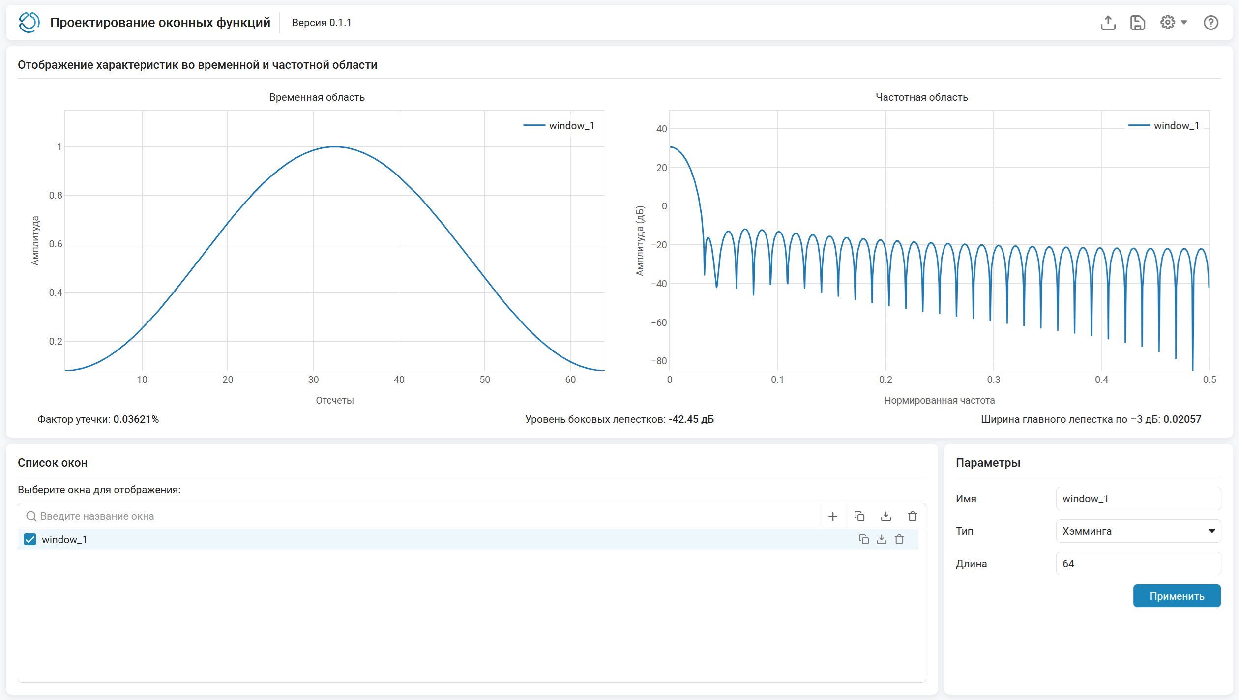
Using the app, you can:
-
Calculate and analyze characteristics in the frequency and time domains for parametric and nonparametric window functions;
-
Visualize the characteristics in the time and frequency domain for one or more windows;
-
Import and export the application configuration (session);
-
Save the calculated window coefficients as a variable workspace, a separate file (extensions CSV, TXT, JLD2, MAT) and an executable jl file.
Working with the app
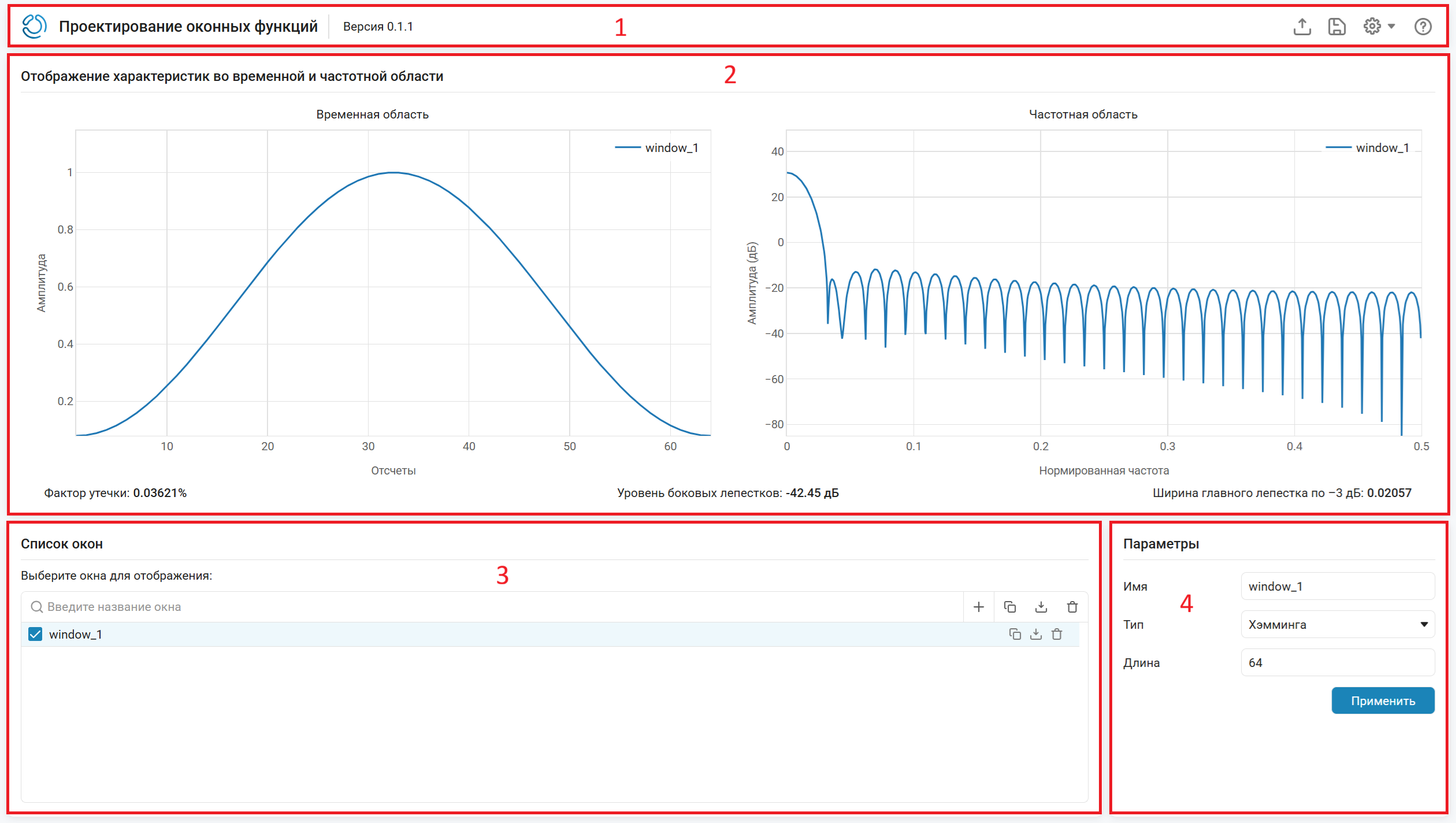
Four sections are used to work with the application.:
-
Toolbar (1) — a section for global management of the current session: On the right is a block of control elements that ensure the import of previously saved sessions, export calculated coefficients to files of various formats or save the session, access the chart display settings menu, as well as direct access to documentation. Engee. The application name and its current version number are displayed on the left side of the section.
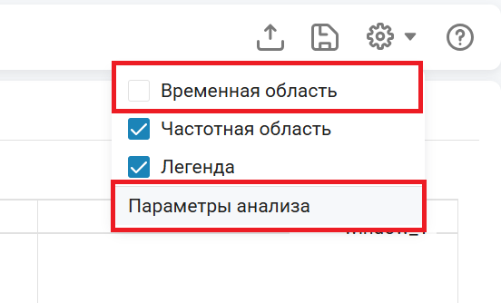
There are three checkboxes in the display settings menu: two of them affect the display of graphs in the visualization area, and the third one affects the display of the legend on these graphs. This menu also contains the analysis parameters, for more information, see Parameters.
-
Visualization area (2) is a central section designed for simultaneous analysis of the characteristics of selected window functions in the time and frequency domains displayed on two interactive graphical windows: «Time domain» and «Frequency domain» accordingly.
Numerical quality metrics calculated for the current characteristics of the window are located under the graphic fields.:
-
Leakage factor — characterizes the degree of spectral spreading and is expressed as a percentage of the signal energy falling on the side lobes of the spectrum of the window;
-
Side lobe level — characterizes the maximum level of the side lobe relative to the main maximum of the amplitude-frequency response (frequency response) and is expressed in dB;
-
The width of the main lobe by −3 dB — characterizes the width of the spectrum of the window function by level
−3dB and is expressed in frequency units or normalized frequency units.
-
-
Window List (3) is an interactive manager of created window functions. On the panel, you can find a window by name, add a new window, copy or delete an existing one, and upload the calculated weights to the workspace. Engee.
-
Parameters (4) is the section where the parameter values are set. Each parameter has a default value that can be changed.
The Parameters section contains all available application parameters with explanations.
Parameters
The following is an overview of the application settings.
# Name is the name of the window
+
window_1 (by default) | line
Details
Specify the name of the window function. The name must be non-empty and unique among all windows in the current session.
# Type — window type
+
Hamming (by default) | With a flat top | Bartlett’s | Bartlett-Hanning | Blackman’s | Blackman-Harris | Bomana | Gauss | The Kaiser | Nattala | Parzen | Rectangular | Taylor’s | Triangular | Tukey | Hannah (Henning) | Chebysheva | Custom
Details
Select the type of window function:
-
With a flat top— a nonparametric window, the coefficients of which are calculated using the formulawhere , , , , (for more information, see
flattopwin); -
Bartlett’s— a nonparametric window, the coefficients of which are calculated using the formula(for more information, see
bartlett); -
Bartlett-Hanning— a nonparametric window, the coefficients of which are calculated using the formula(for more information, see
barthannwin); -
Blackman’s— a nonparametric window, the coefficients of which are calculated using the formula(for more information, see
blackman); -
Blackman-Harris— a nonparametric window, the coefficients of which are calculated using the formulawhere , , , (for more information, see
blackmanharris); -
Bomana— a nonparametric window, the coefficients of which are calculated using the formula(for more information, see
bohmanwin); -
Gaussis a parametric window, the coefficients of which are calculated using the formula(for more information, see
gausswin); -
The Kaiseris a parametric window, the coefficients of which are calculated using the formula(for more information, see
kaiser); -
Nattala— a nonparametric window, the coefficients of which are calculated using the formulawhere , , , (for more information, see
nuttallwin); -
Parzen— a nonparametric window, the coefficients of which are calculated using the formula(for more information, see
parzenwin); -
Rectangular— a nonparametric window, the coefficients of which are calculated using the formula(for more information, see
rectwin); -
Taylor’sis a parametric window, the coefficients of which are calculated using the formula(for more information, see
taylorwin); -
Triangular— a nonparametric window, the coefficients of which are calculated using the formula(for more information, see
triang); -
Tukeyis a parametric window, the coefficients of which are calculated using the formula(for more information, see
tukeywin); -
Hannah (Henning)— a nonparametric window, the coefficients of which are calculated using the formula(for more information, see
hann); -
Hamming(by default) is a nonparametric window, the coefficients of which are calculated using the formula(for more information, see
hamming); -
Chebyshevais a parametric window, the coefficients of which are calculated using the formulawhere (for more information, see
chebwin); -
Custom— allows you to set an arbitrary window function by writing Julia code in the EngeeCode field. It can be implemented in various forms.:-
An analytical expression is a compact formula that defines the coefficients directly. For example, the expression
abs.(cos.(π * (0:N−1) / N))creates a cosine window. -
The list generator is more complex constructions with logic. For example,
[i < N/2 ? 1.0 : exp(−(i−N/2)^2 / (N/4)^2) for i in 1:N]creates a window with a flat center and Gaussian drops at the edges. -
Calling custom functions is a function defined in the workspace. Engee, can be called from user code.
The user code is executed in the current session Engee and has access to all its variables and functions. To keep the session portable, it is recommended to use only the variable N. The code is saved along with the session in text form.
-
You can use text input in the field to speed up the search for the desired value among a large number of options.
# Length is the length of the window
+
64 (by default) | scalar
Details
The discrete length of the window function in samples, specified as a positive integer.
# α is the width coefficient
+
2.5 (by default) | scalar
Details
The width coefficient, set as a positive real scalar. Parameter inversely proportional to the width of the window.
Dependencies
To use this parameter, set the Type parameter to Gauss.
# β — form factor
+
0.5 (default) | scalar
Details
The coefficient of the shape, given as a positive real scalar. Parameter it affects the weakening of the side lobes of the Fourier transform of the window.
Dependencies
To use this parameter, set the Type parameter to The Kaiser.
# nbar — the number of side lobes at an almost constant level
+
4 (by default) | scalar
Details
The number of side lobes of an almost constant level adjacent to the main lobe, set as a positive integer. These side lobes are considered «almost constant level» because there is some attenuation in the transition region.
Dependencies
To use this parameter, set the Type parameter to Taylor’s.
# sll — the maximum level of the side lobes relative to the peak of the main lobe
+
−4 (by default) | scalar
Details
The maximum level of the side lobes relative to the peak of the main lobe, set as a real negative scalar in dB. It creates side lobes with peaks on the sll dB is below the peak of the main lobe.
Dependencies
To use this parameter, set the Type parameter to Taylor’s.
# r — cosine fraction
+
0.5 (by default) | scalar
Details
A cosine fraction defined as a real scalar. The Tukey window is a rectangular window in which the first and last r/2 percentages of samples are equal to fractions of a cosine. For example, when r = 0.5 it turns out to be a Tukey window in which 1/2 the entire length of the window consists of segments of a phase-shifted cosine with a period 2r = 1. If you ask r ≤ 0, returns N-dotted rectangular window. If you ask r ≥ 1, returns N- Hannah’s point window.
Dependencies
To use this parameter, set the Type parameter to Tukey.
# r — attenuation of the side lobes
+
100 (by default) | scalar
Details
The attenuation of the side lobes in dB, set as a positive integer. The Chebyshev window has the amplitude of the Fourier transform by r dB is lower than the amplitude of the main lobe.
Dependencies
To use this parameter, set the Type parameter to Chebysheva.
# EngeeCode — text field
+
Details
Enter the code in Julia to set an arbitrary window function. The calculation of the entered expression should return a vector of real coefficients of the window of the specified length. A predefined variable is available in the expression , corresponding to the current value of the Length parameter.
Dependencies
To use this field, set the Type parameter to Custom.
parameters of analysis
# Number of points — number of FFT points
+
1024 (by default) | scalar
Details
The number of FFT points used to calculate the frequency response, set as an integer.
Minimum allowed value: 2. Increasing this parameter smooths out the spectrum, which makes it possible to examine the shape of the main lobe and the side lobes in more detail. However, excessive magnification (for example, more 4096) may slow down the recalculation of graphs. Recommended value: 1024–2048 for most practical tasks.
# Range — frequency range
+
The positive half is [0, π) (by default) | Full range [0, 2π) | Symmetric [-π, π)
Details
The frequency range displayed on the frequency domain graph is set by one of the following values:
-
The positive half is [0, π)— the standard mode for analyzing the spectrum of real signals, since the amplitude characteristic is symmetrical; it represents a range from0up to the Nyquist frequency ( Hz or0.5standardized units); -
Full range [0, 2π)— useful for observing the periodicity of the spectrum, but is not usually used to estimate the window parameters; it is a range from0before (1.0standardized units); -
Symmetric [-π, π)— provides a visual representation of the symmetry of the spectrum relative to the zero frequency; represents the range from before (from−0.5before0.5standardized units).This mode is incompatible with the logarithmic frequency scale; if you try to use them together, the system will give an error.
# Response — type of amplitude response
+
Amplitude, dB (default) | The amplitude | The square of the amplitude | The zero phase
Details
The type of amplitude response displayed on the ordinate axis of the frequency graph, set by one of the following values:
-
The amplitude— linear amplitude (dimensionless), useful for estimating absolute values, but small-amplitude side lobes may be poorly visible; -
Amplitude, dB— amplitude in dB , allows you to simultaneously see both the main lobe and the side lobes with a large dynamic range (up to−100dB and below); -
The square of the amplitude— displays the power of the spectrum, used in energy spectrum estimation tasks; -
The zero phase— displays the amplitude taking into account the phase shift, but for symmetrical windows this mode is equivalent toThe amplitude.
# Frequency scale — the type of scaling of the frequency axis
+
Linear (by default) | Logarithmic
Details
The type of scaling of the frequency axis, set by one of the following values:
-
Linear— uniform linear scale; -
Logarithmic— logarithmic scale, allows you to examine in detail the low frequency region, where the side lobes are often concentrated.This type is incompatible with a symmetric range; if you try to use them together, the system will return an error.
# Frequency units — units of frequency measurement
+
Normalized (by default) | Hz | kHz | MHz | GHz
Details
The physical meaning of the abscissa axis of the frequency graph, given by one of the following values:
-
Normalized— the frequency is expressed in fractions of the Nyquist frequency (from0before0.5for the positive half); -
Hz,kHz,MHz,GHz— frequency is expressed in Hz or multiples of units. When selecting this option, you must specify the value of the parameter Sampling rate. The width of the main lobe and other frequency-dependent metrics will be recalculated in Hz.
#
Sampling rate —
Sampling
rate
1 (by default) | scalar
Details
The value used to recalculate the normalized frequencies in Hz and to calculate the width of the main lobe in Hz, set as a positive finite number.
Dependencies
To use this parameter, set the Frequency Units parameter to a value other than Normalized.
# Normalize amplitude — control of amplitude normalization
+
Details
Select this option to bring the maximum value of the spectrum amplitude to 1 on a linear scale or to 0 dB in logarithmic. This is useful when comparing windows with different energies, as it allows you to focus on the shape of the spectrum rather than on absolute levels.
Examples
Side lobes of the Hamming window
Details
Visualize the side lobes of the Hamming window with the length 64 the countdown.
-
In the upper-right corner, open the Display Settings menu, uncheck the Time domain checkbox, and click the Analysis Options button.:
-
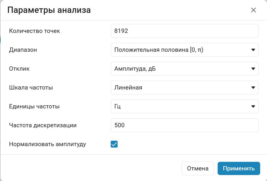
In the dialog box, specify the following parameters:
-
Let’s set the value for the parameter Number of points
8192. -
Set the parameter Frequency units to
Hz. -
Set the parameter Sampling rate to
500. -
Check the box Normalize the amplitude.
-
-
Click the Apply button to close the dialog box. On the panel visualization window tools select the Scale option and select the area on the graph from
10before35Hz to examine in detail the first two side lobes of the window.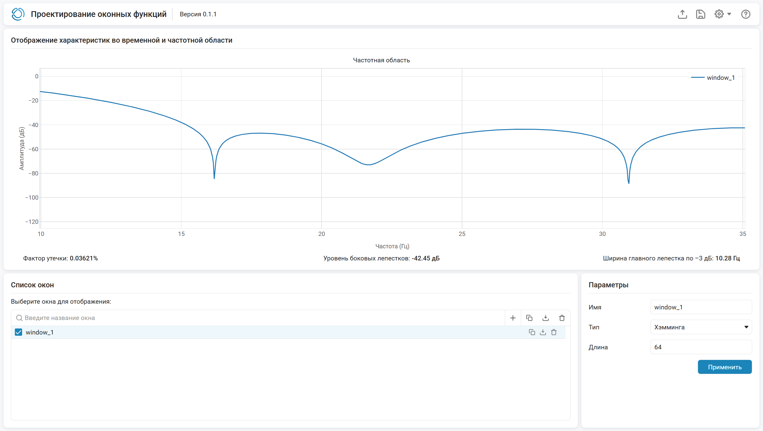
Boman’s Window
Details
Let’s set the Boman window to be long 128 and export it to the workspace. Engee.
-
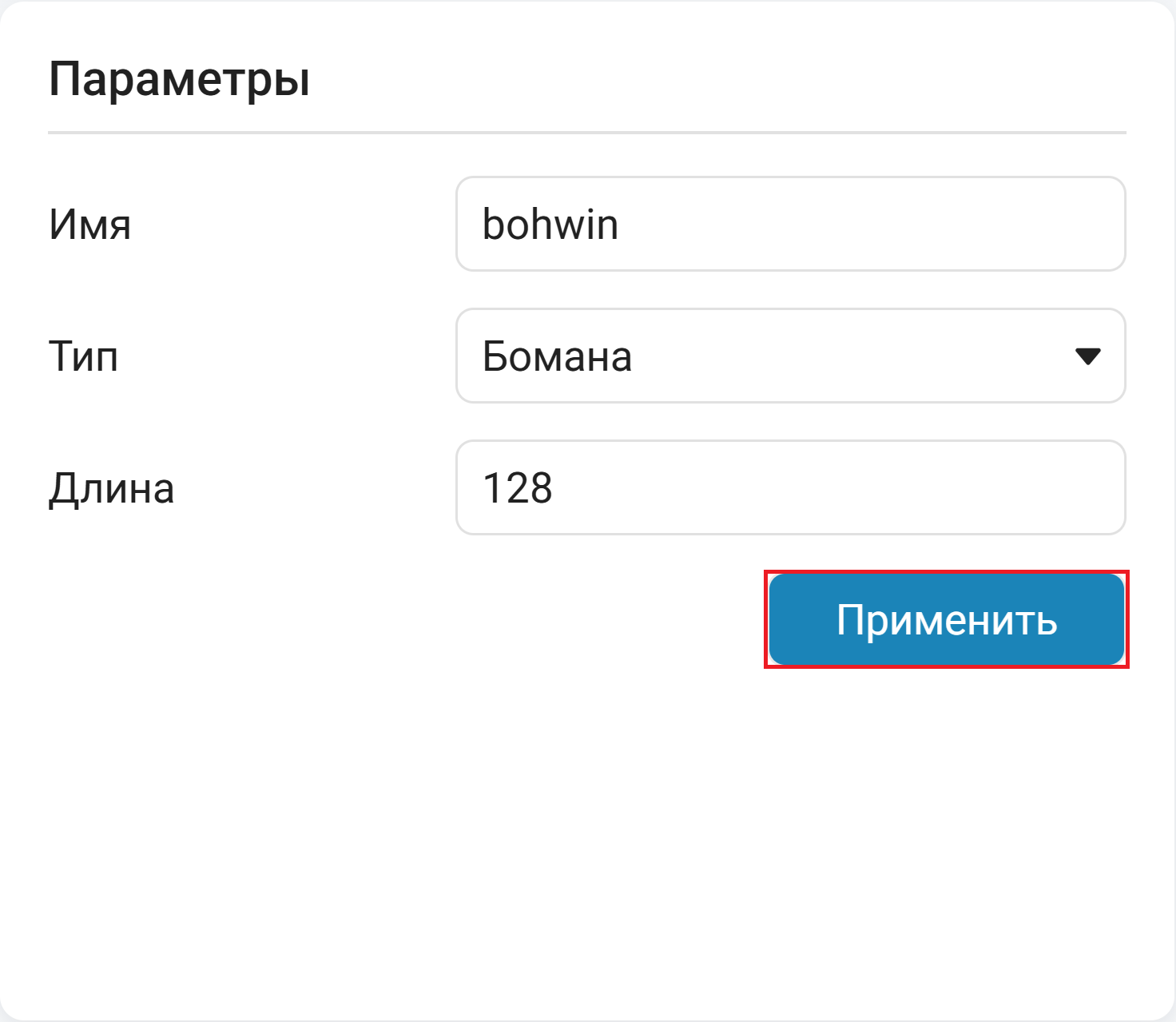
Let’s create a Boman window, in the Parameters section:
-
Setting the value for the Type parameter
Bomana. -
Setting the Length parameter to
128. -
Setting the value for the Name parameter
bohwin.
-
-
Click Apply.
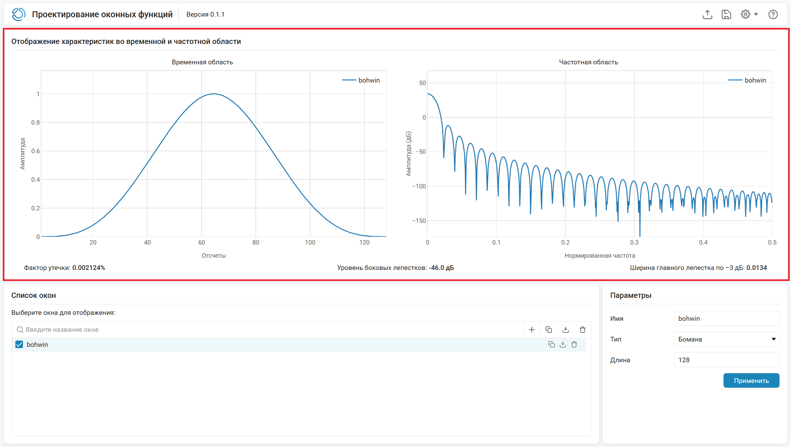
The graphs in the time and frequency domains will be updated in the characteristics display window.:
-
Click the Save button
 , located in the upper right corner. In the window that opens, click Export:
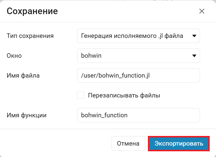
We will receive the following message:
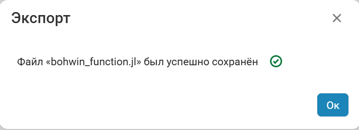
-
File
bohwin_function.jlThe generated code can be found in the file browser. Engee. Its contents:# Generated executable window function # name: bohwin # type: Бомана import EngeeDSP function bohwin_function() N = 128 return EngeeDSP.Functions.bohmanwin(N) end
Based on the obtained function, we construct graphs in Engee. Connect the window calculation file.
include("bohwin_function.jl");Let’s record the window counts in a variable wind and let’s build a graph in the time domain.
wind = bohwin_function()

plot(wind, xlab = "Отсчеты", ylab = "Амплитуда", title = "Окно Бомана", lab="")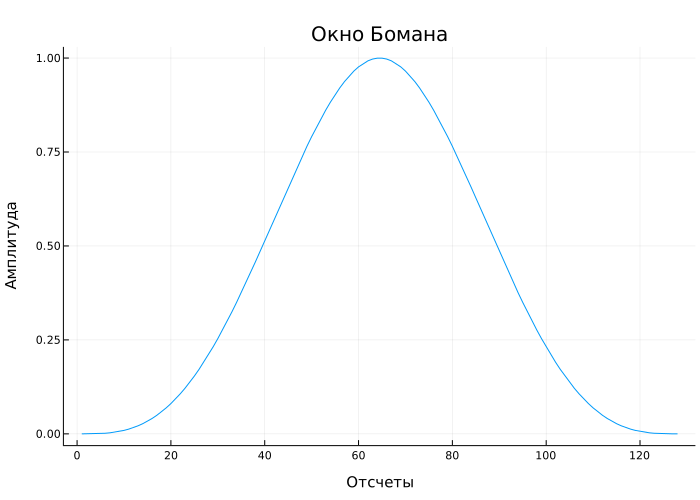
Let’s calculate and build a two-way spectrum.
len_fft = 1024
spec_wind = EngeeDSP.Functions.fft(wind, len_fft) # расчет спектра

f_grid = (0:(len_fft-1)) ./ len_fft
plot(f_grid, 10log10.(abs.(spec_wind)), xlab = "Нормированная частота",
     ylab = "Амплитуда", title="Двухсторонний спектр", lab="")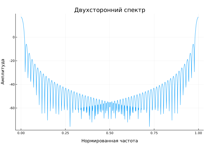
As well as a one-way spectrum.
len_fft_2 = 512
plot(f_grid[1:len_fft_2], 10log10.(abs.(spec_wind[1:len_fft_2])),
     xlab = "Нормированная частота", ylab = "Амплитуда",
     title = "Односторонний спектр", lab="")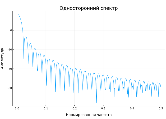
Kaiser Windows
Details
Let’s examine the behavior of the Kaiser window, depending on the length and form factor. .
-
Let’s create a Kaiser window, in the Parameters section:
-
Setting the value for the Type parameter
The Kaiser. -
Setting the Length parameter to
20. -
Let’s set the β parameter to
0.0. -
Setting the value for the Name parameter
kaiser0.
-
-
Click Apply. The graphs in the time and frequency domains will be updated in the characteristics display window.:
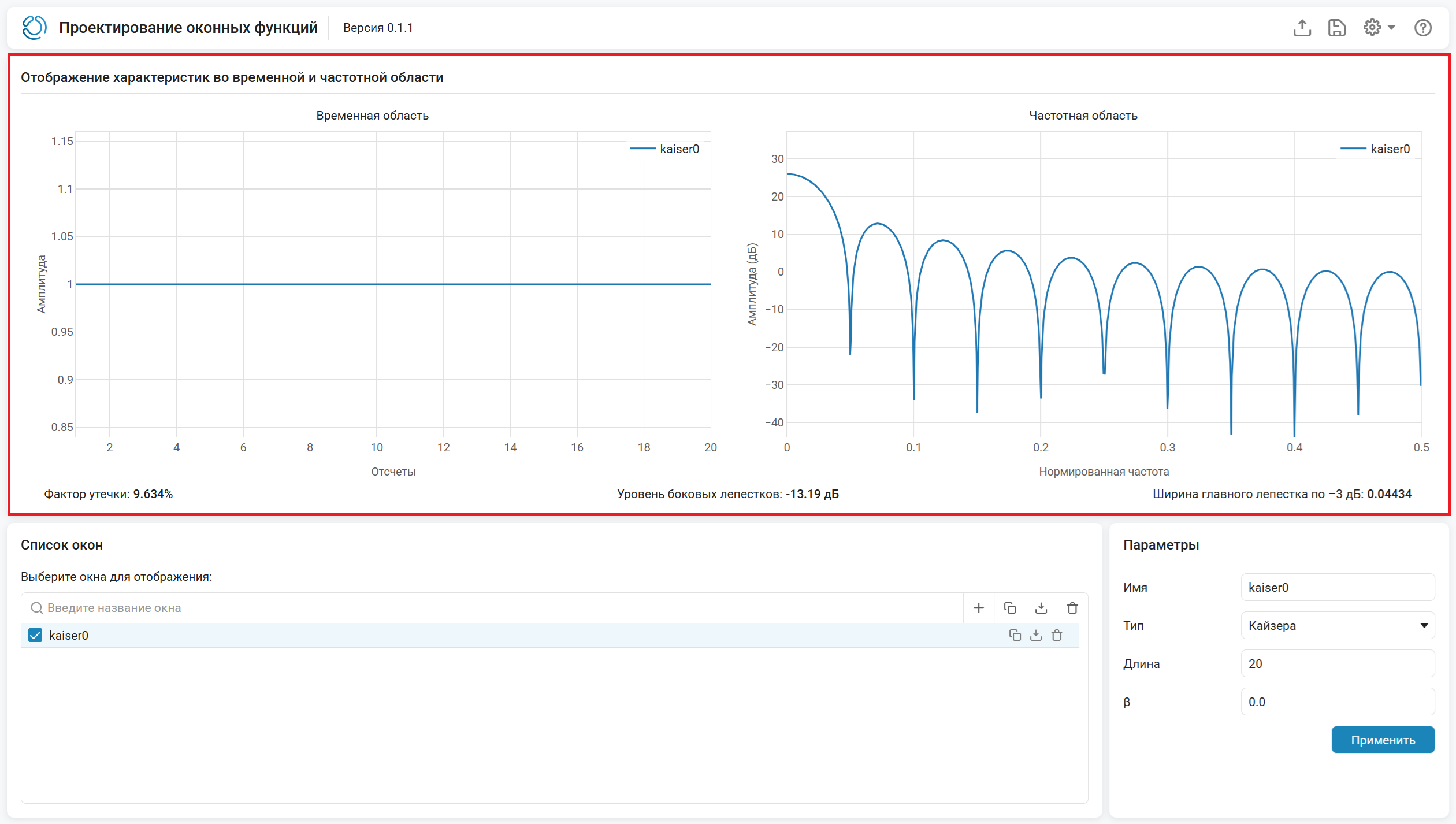
-
In the List of windows section, click the Add Window button:
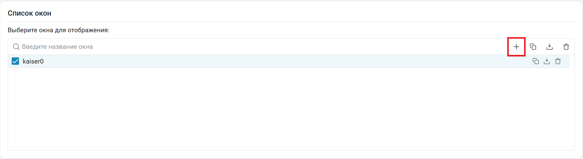
Similarly, we will create a Kaiser window with a length of
20with the parameter . Let’s call the windowkaiser3and click Apply. We get: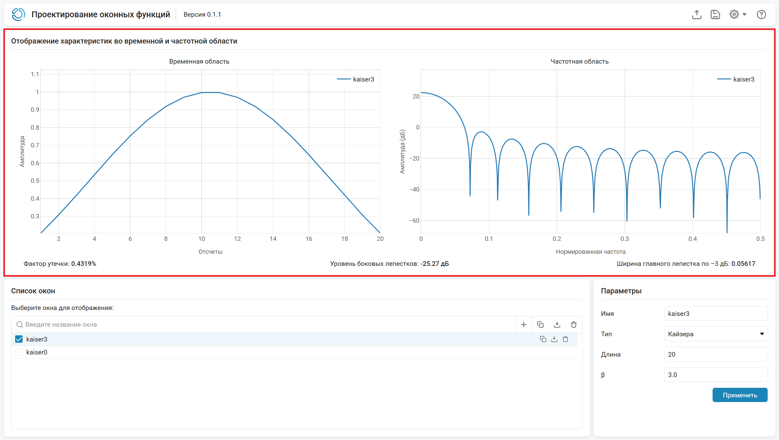
-
In the List of Windows section, click Duplicate the selected window (or Duplicate):
to create a third Kaiser window
kaiser6with the parameter . Click Apply.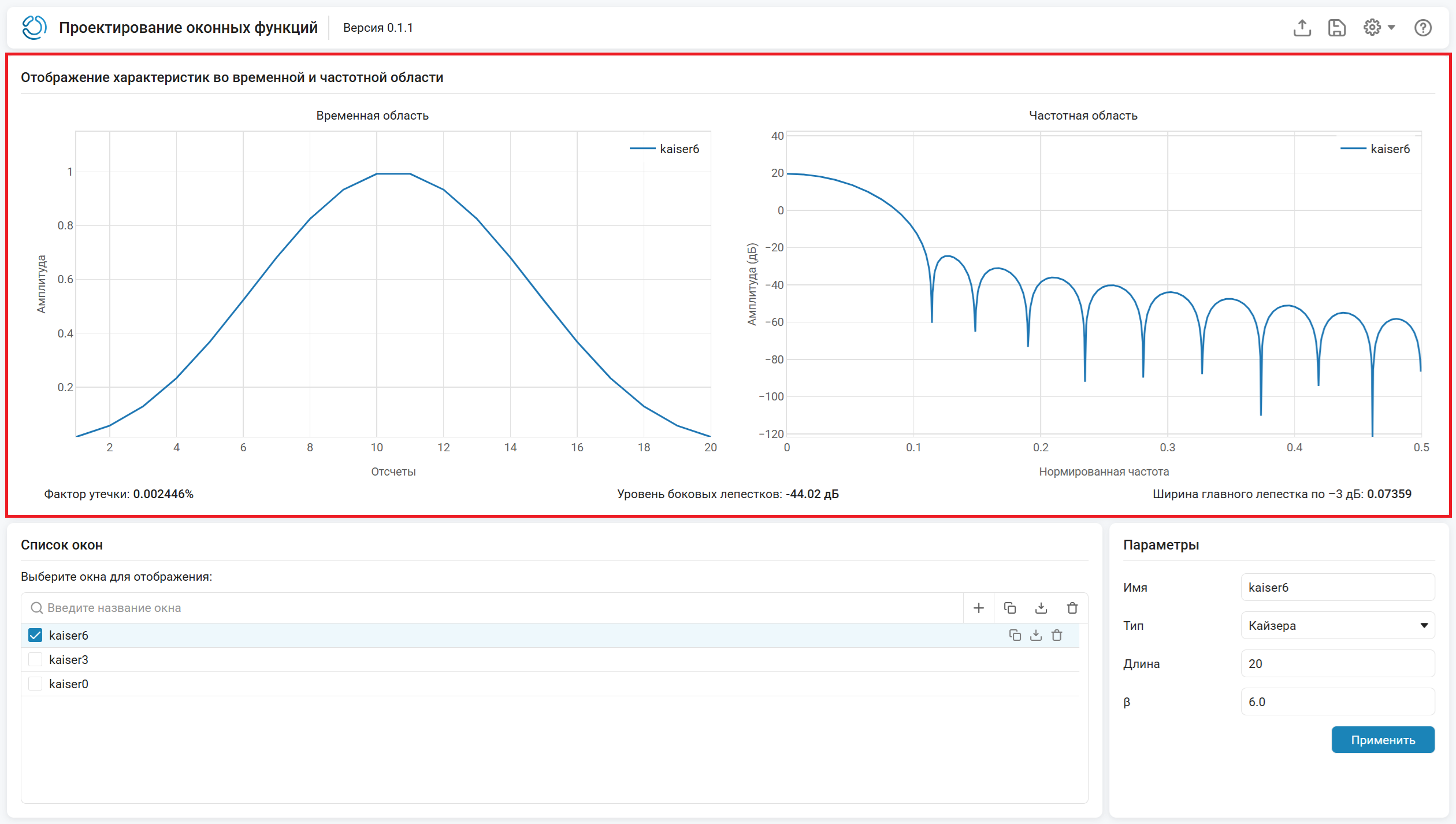
-
In the section List of windows select three windows, then all graphs will be displayed in the section Display of characteristics in the time and frequency domain:
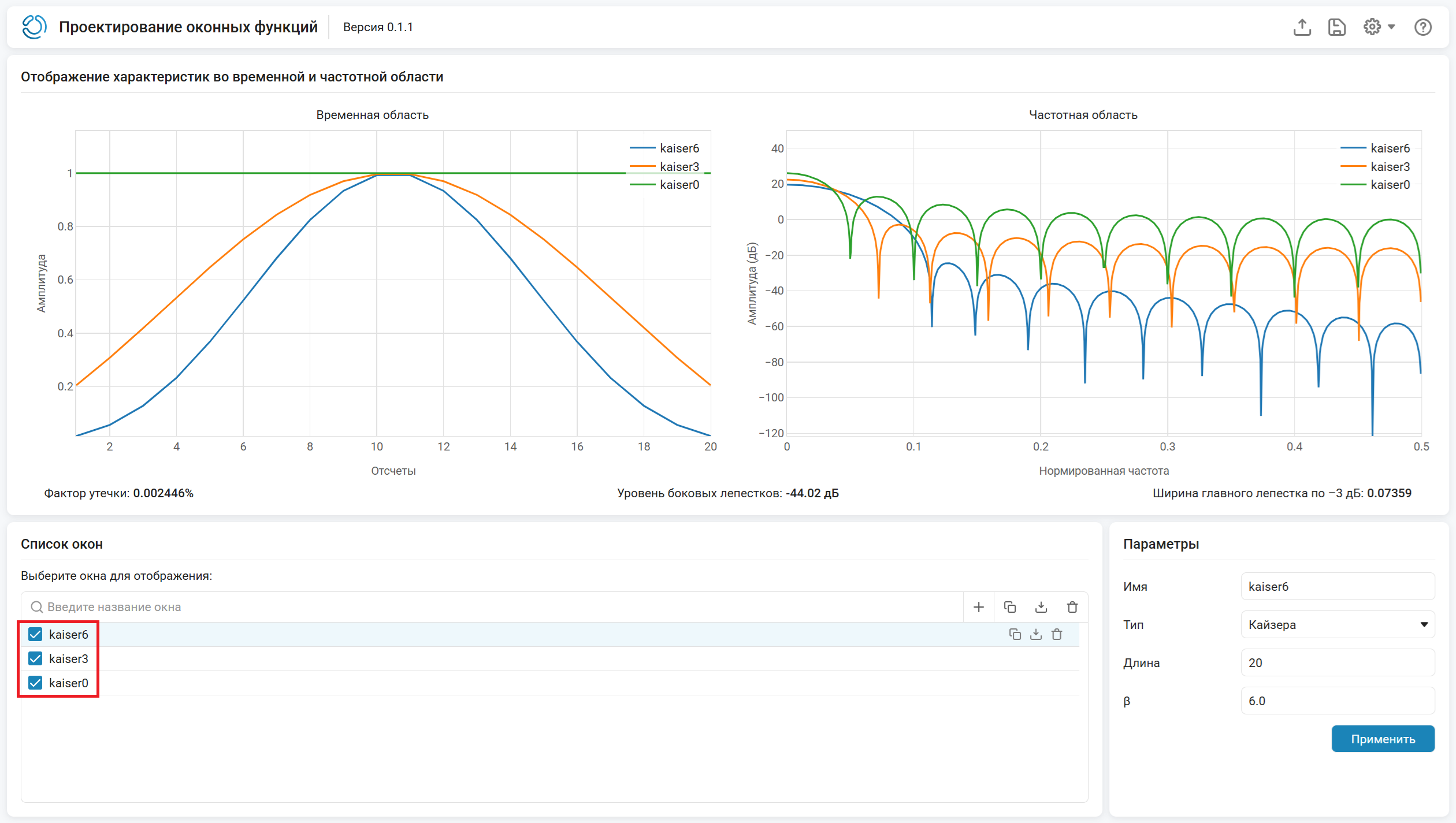
-
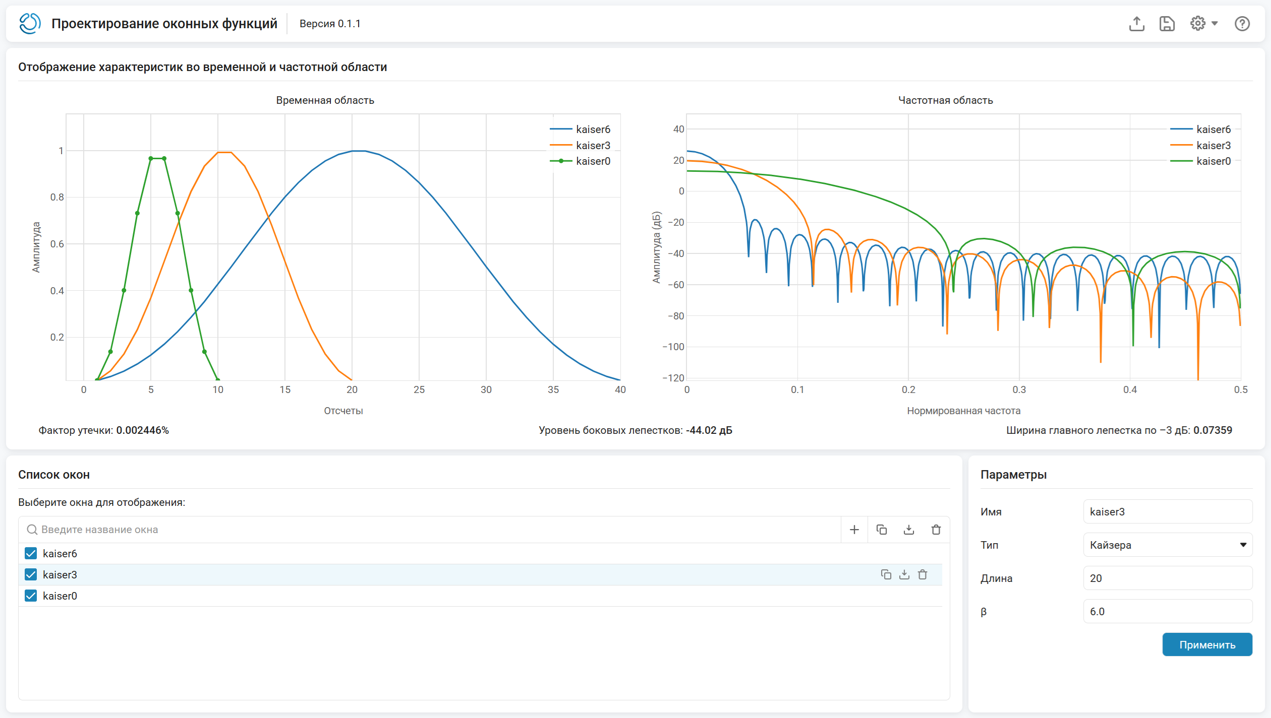
Let’s change the parameter values for each window:
-
Choose
kaiser0and set the Length parameter to10, and for β —6.0. Click Apply. -
Choose
kaiser3and set the β parameter to6.0. Click Apply. -
Choose
kaiser6and set the Length parameter to40. Click Apply.
-