Pressure characteristics of the compressor

The example illustrates a tabular method for setting the pressure characteristics of a compressor through the degree of pressure increase, the specified mass flow rate and efficiency, and calculating acceleration dynamics based on these characteristics.

Data preparation

In the files compressor_map_speed_lines and compressor_map_efficiency_data The lines of the compressor pressure map are contained - contour points in terms of rotation speed and efficiency.

]add JLD2, Interpolations, ScatteredInterpolation

using JLD2, Interpolations, ScatteredInterpolation

@load "compressor_map_speed_lines.jld2"

# Creation of matrices for the reduced mass flow rate and degrees of pressure increase
mdot_TLU = [Line1000[:,1]'; Line1500[:,1]'; Line2000[:,1]'; Line2500[:,1]'; Line3000[:,1]'; Line3500[:,1]']
pr_TLU   = [Line1000[:,2]'; Line1500[:,2]'; Line2000[:,2]'; Line2500[:,2]'; Line3000[:,2]'; Line3500[:,2]']
# Creating a reduced velocity vector
omega_TLU = [1000, 1500, 2000, 2500, 3000, 3500]
# Beta varies from 0 to 1. Length = number of points on each line
beta_TLU = range(0, 1, length=7)

@load "compressor_map_efficiency_data.jld2"
# Add another point in the middle of the characteristic to avoid an intersection.
Eff80 = [Eff80[1:3,:]; [0.55 1.5]; Eff80[4:end, :]]
# Organizing efficiency data for use with interpolation
eff_levels = [(Eff80, 0.80), (Eff82, 0.82), (Eff84, 0.84), (Eff86, 0.86), (Eff88, 0.88), (Eff90, 0.90)]

# Output of a graph with compressor characteristics
include("create_compressor_map.jl")
p, eta_TLU = create_compressor_map(mdot_TLU, pr_TLU, omega_TLU, eff_levels)
plot!(p)

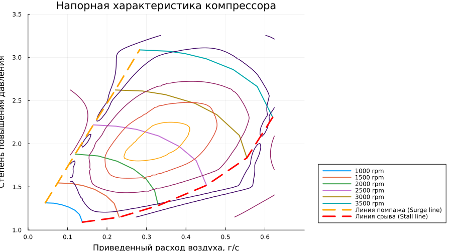
The contour graph shows that the interpolated efficiency contours almost match the original data. In addition, the points are now presented in a format that can be used in the Compressor block.

At first, the characteristic had overly simplified contours, so we interpolated the efficiency isolines, and then interpolated over a thinner, uniform grid of values, selecting a suitable core for smoothing.

There may be a loss of accuracy during interpolation. The only reliable way to avoid this loss of accuracy is to use more accurate raw data. Please note that the data is set in an auxiliary coordinate system determined by the reduced rotation frequency and the auxiliary coordinate β.

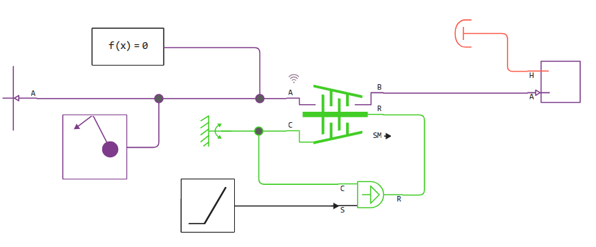
Compressor calculation

In this project, we set the parameters of the Compressor (D) block from the workspace using variables generated based on the initial tabular data.:

omega_TLU
beta_TLU
pr_TLU
mdot_TLU
eta_TLU

The operating temperature and pressure values are equal to the inlet tank temperature and atmospheric pressure. Therefore, the values of the reduced mass flow rate and the reduced rotational speed coincide with the actual values for the source of the ideal angular velocity (since the correction factor is one).

Let's see how an increase in the compressor's rotation speed leads to an increase in pressure in a constant volume chamber.

engee.open("compressor_map_example.engee")
data = engee.run();

# The temperature and pressure are already equal to the operating values, they do not need to be specified.
mdot_corrected = data["Compressor (G).mdot_inlet"].value .* 1000; # The property is stored in kg/s
PR = data["Compressor (G).outlet.p"].value ./ data["Compressor (G).inlet.p"].value;

# We display the transition mode line on top of the previous chart
plot!(mdot_corrected, PR, lw=3, label="Pickup line", lc=:black, ls=:dash)

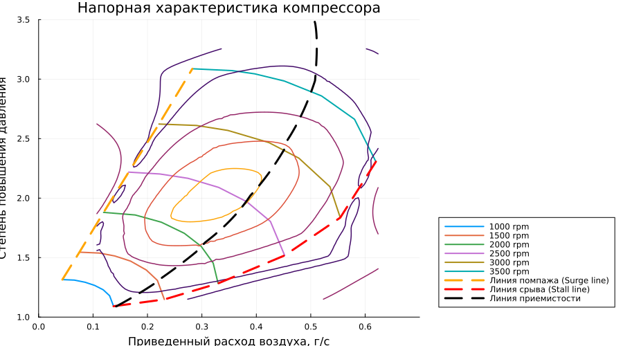
Conclusion

The compressor characteristics match well with the initial data. The interpolation process causes some error, but it can be minimized by improving the approach to data preprocessing or simply increasing their number.