Classification
This example shows how to perform classification using naive Bayesian classifiers and decision trees. Suppose you have a dataset containing observations with measurements of various variables (called predictors) and their known class labels. When getting predictor values for new observations, can you determine which classes these observations are likely to belong to? This is the problem of classification.
An internet connection is required to run this demo
Fischer's Irises
The Fischer's Irises dataset consists of measurements of the length and width of the sepals, as well as the length and width of the petal for 150 specimens of irises. There are 50 samples of each of the three species. Upload the data and see how the sepals differ in size from one species to another. You can use the first two columns containing their dimensions.
Downloading libraries for statistical analysis
To work with statistical data, you need to download the specified libraries.
Pkg.add(["RDatasets", "NaiveBayes", "StatsBase", "StatsPlots", "DecisionTree", "ScikitLearn"])
Pkg.add("DecisionTree")# loading the library of decision trees
Pkg.add("NaiveBayes")# loading a library with Bayesian classifiers
Pkg.add("StatsBase")# to use predict in the Bayesian classifier
Pkg.add("StatsPlots")# for plotting point graphs
Connecting downloaded and auxiliary libraries for uploading a dataset, for plotting graphs, and for training classifiers.
using NaiveBayes
using RDatasets
using StatsBase
using Random
using StatsPlots
using Plots, RDatasets
using DecisionTree
using ScikitLearn: fit!, predict
using ScikitLearn.CrossValidation: cross_val_score
Formation of predictor matrices and a set of class labels.
features, labels = load_data("iris")
features = float.(features);
labels   = string.(labels);
Enabling the Plots library method to display graphs, as well as defining a dataset to display the distribution of observations across the width and length of the sepal (SepalWidth, SepalLength).
plotlyjs();
iris = dataset("datasets", "iris");
A dataset with predictors and classes.
first(iris[:,1:5],5)
Graph of the distribution of observations by the width and length of the sepals.
@df iris scatter(:SepalLength, :SepalWidth, group = :Species)
Preparation of a predictor matrix for all hypothetical observations, which will be needed when constructing a dot graph showing the classifier's work on dividing objects into classes.
h = 10000;
x1 = rand(4:0.1:8, h)
x1t = x1'
x2 = rand(2:0.1:4.5, h)
x2t = x2'
x12 = vcat(x1t,x2t);
Naive Bayesian Classifier
The Naive Bayes Classifier is a simple probabilistic classifier based on the application of Bayes' theorem with strict (naive) independence assumptions.
The advantage of the naive Bayesian classifier is the small amount of data needed for training, parameter estimation, and classification.
Preprocessing of data for use in training the Baesian classifier model.
Xx = Matrix(iris[:,1:2])';#features';#
Yy = [species for species in iris[:, 5]];# labels;
p, n = size(Xx)
train_frac = 0.8
k = floor(Int, train_frac * n)
idxs = randperm(n)
train_idxs = idxs[1:k];
test_idxs = idxs[k+1:end];
Determination of the model structure by GaussianNB method and its training by fit method.
Calculating accuracy.
modelNB = GaussianNB(unique(Yy), p)
fit(modelNB, Xx[:, train_idxs], Yy[train_idxs])
accuracyNB = count(!iszero, StatsBase.predict(modelNB, Xx[:,test_idxs]) .== Yy[test_idxs]) / count(!iszero, test_idxs)
println("Accuracy: $accuracyNB")
Forming a forecast matrix for new observations.
predNB = fill("", 0);# Defining an empty array
predNB = (NaiveBayes.predict(modelNB, x12[:,1:h]));# filling an array with prediction values
Forming a predictor-forecast matrix for new observations.
x_pred_NB = hcat(x12',predNB);
pred_df_NB = DataFrame(x_pred_NB,:auto);
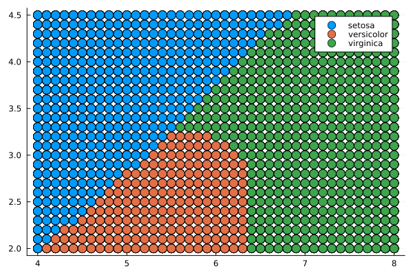
Displaying the classifier's division of the predictor field into classes corresponding to the types of irises.
gr()
@df pred_df_NB scatter(:x1, :x2, group = :x3, markersize = 7)
Decision tree
The decision tree is a set of simple rules such as "if the sepals are less than 5.45 in length, classify the sample as setosa". Decision trees are also nonparametric because they do not require any assumptions about the distribution of variables in each class.
The process of building decision trees consists in the sequential, recursive division of the training set into subsets using decision rules at the nodes.
Determination of the model structure by the DecisionTreeClassifier method and its training by the fit! method.
Calculating accuracy using cross-validation.
Displaying the decision tree.
modelDT = DecisionTreeClassifier(max_depth=10)# defining the model structure
fit!(modelDT, features[:,1:2], labels)# model training
print_tree(modelDT, 5)# displaying the decision tree
accuracy = cross_val_score(modelDT, features[:,1:2], labels, cv=8)# calculating accuracy
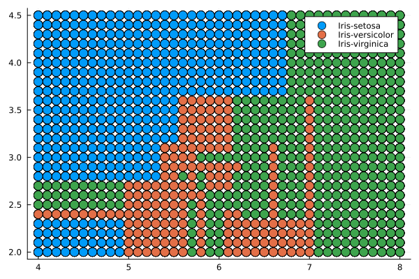
This random-looking tree uses a set of rules like "Feature 1 < 5.55" to classify each sample according to one of the 11 end nodes. To determine the type of the observed iris, start with the upper condition and apply the rules. If the observation satisfies the rule, you choose the upper branch, and if not, then choose the lower one. As a result, you will reach the end node, which will assign the observed instance a value of one of three types.
Forming a forecast matrix for new observations.
predDT = fill("", 0);# defining an array
# formation of the value-prediction matrix for the decision tree
for i in 1:h
    predDT = vcat(predDT, predict(modelDT, x12[:,i]))
end
Forming a predictor-forecast matrix for new observations.
x_pred_DT = hcat(x12',predDT);
pred_df_DT = DataFrame(x_pred_DT,:auto);
Displaying the classifier's division of the predictor field into classes corresponding to the types of irises.
@df pred_df_DT scatter(:x1, :x2, group = :x3, markersize = 7)
Conclusion
In this example, the classification problem was solved using a naive Bayesian classifier and a decision tree. The use of the DecisionTree and NaiveBayes libraries was demonstrated.
They were used to train classifiers.
The classifiers, in turn, with a fairly small data set, showed good accuracy and divided the predictor field into classes.