Engee documentation
Notebook

Training a fully connected multi-layered neural network on corrected data

In this example, we will consider data processing and training based on a neural network model. The sliding window method will be demonstrated to divide the training and test samples into training datasets, and model parameters will be determined to obtain the most accurate predicted values.

Launching the necessary libraries:

In [ ]:
Pkg.add(["Statistics", "CSV", "Flux", "Optimisers"])
   Resolving package versions...
  No Changes to `~/.project/Project.toml`
  No Changes to `~/.project/Manifest.toml`
In [ ]:
using Statistics
using CSV
using DataFrames
using Flux
using Plots
using Flux: train!
using Optimisers

Preparation of training and test samples:

Uploading data for model training:

In [ ]:
df = DataFrame(CSV.File("$(@__DIR__)/data.csv")); 

The data was saved after executing the example /start/examples/data_analysis/data_processing.ipynb.

Formation of a training data set:

The entire dataset was divided into a training and a test sample. The training sample was 0.8 of the total dataset, and the test sample was 0.2.

In [ ]:
T = df[1:1460,3]; # определение обучающего набора данных, весь датасет 1825 строк
first(df, 5)
Out[0]:
5×3 DataFrame
RowdatePT
Int64Float64Float64
11747.719.7
22744.222.1
33748.623.0
44754.523.4
55754.621.9

Dividing the vector T into batches of 100 observations in length:

In [ ]:
batch_starts = 1:1:1360 # определение диапазона для цикла

weather_batches = [] # определение пустого массива для записи результатов выполнения цикла
for start in batch_starts
    dop = T[start:start+99] # батч на текущем временном шаге
    weather_batches = vcat(weather_batches, dop) # запись батча в массив
end

A batch is a small data set that can serve as a training set for building a forecasting model. Taken from the initial training set T using the sliding window method.

Sliding window method:

image.png

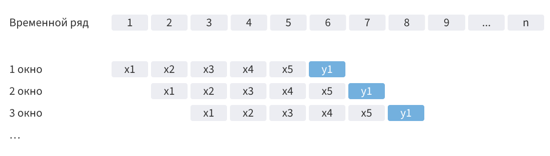
where x is the observation and y1 is the predicted value.

Converting the resulting set into a vector string:

In [ ]:
weather_batches = weather_batches'
Out[0]:
1×136000 adjoint(::Vector{Any}) with eltype Any:
 19.7  22.1  23.0  23.4  21.9  23.35  …  26.4  18.8  19.7  16.3  16.8  20.5

Changing the shape of the array to match the length of the batch specified above:

In [ ]:
weather_batches = reshape(weather_batches, (100,:))
Out[0]:
100×1360 reshape(adjoint(::Vector{Any}), 100, 1360) with eltype Any:
 19.7   22.1   23.0   23.4   21.9   23.35  …  -4.4     -2.9  -4.0  -4.7  -4.2
 22.1   23.0   23.4   21.9   23.35  24.8      -2.9     -4.0  -4.7  -4.2  -7.8
 23.0   23.4   21.9   23.35  24.8   26.25     -4.0     -4.7  -4.2  -7.8   1.7
 23.4   21.9   23.35  24.8   26.25  27.7      -4.7     -4.2  -7.8   1.7   2.8
 21.9   23.35  24.8   26.25  27.7   28.0      -4.2     -7.8   1.7   2.8   2.9
 23.35  24.8   26.25  27.7   28.0   27.4   …  -7.8      1.7   2.8   2.9   5.8
 24.8   26.25  27.7   28.0   27.4   25.1       1.7      2.8   2.9   5.8   3.1
 26.25  27.7   28.0   27.4   25.1   25.6       2.8      2.9   5.8   3.1   4.1
 27.7   28.0   27.4   25.1   25.6   24.5       2.9      5.8   3.1   4.1   5.1
 28.0   27.4   25.1   25.6   24.5   21.9       5.8      3.1   4.1   5.1   4.4
 27.4   25.1   25.6   24.5   21.9   15.5   …   3.1      4.1   5.1   4.4   4.3
 25.1   25.6   24.5   21.9   15.5   22.7       4.1      5.1   4.4   4.3   7.5
 25.6   24.5   21.9   15.5   22.7   23.1       5.1      4.4   4.3   7.5   6.9
  ⋮                                  ⋮     ⋱   ⋮                         
 22.1   18.9   17.9   15.5   20.9   20.3      19.9917  19.7  15.3  20.5  19.5
 18.9   17.9   15.5   20.9   20.3   16.7      19.7     15.3  20.5  19.5  19.3
 17.9   15.5   20.9   20.3   16.7   15.5   …  15.3     20.5  19.5  19.3  21.6
 15.5   20.9   20.3   16.7   15.5   12.7      20.5     19.5  19.3  21.6  21.1
 20.9   20.3   16.7   15.5   12.7    9.7      19.5     19.3  21.6  21.1  23.8
 20.3   16.7   15.5   12.7    9.7    6.7      19.3     21.6  21.1  23.8  23.6
 16.7   15.5   12.7    9.7    6.7    4.3      21.6     21.1  23.8  23.6  26.4
 15.5   12.7    9.7    6.7    4.3    5.6   …  21.1     23.8  23.6  26.4  18.8
 12.7    9.7    6.7    4.3    5.6   12.2      23.8     23.6  26.4  18.8  19.7
  9.7    6.7    4.3    5.6   12.2   12.8      23.6     26.4  18.8  19.7  16.3
  6.7    4.3    5.6   12.2   12.8   12.3      26.4     18.8  19.7  16.3  16.8
  4.3    5.6   12.2   12.8   12.3    9.8      18.8     19.7  16.3  16.8  20.5
In [ ]:
X = weather_batches # переприсвоение
Out[0]:
100×1360 reshape(adjoint(::Vector{Any}), 100, 1360) with eltype Any:
 19.7   22.1   23.0   23.4   21.9   23.35  …  -4.4     -2.9  -4.0  -4.7  -4.2
 22.1   23.0   23.4   21.9   23.35  24.8      -2.9     -4.0  -4.7  -4.2  -7.8
 23.0   23.4   21.9   23.35  24.8   26.25     -4.0     -4.7  -4.2  -7.8   1.7
 23.4   21.9   23.35  24.8   26.25  27.7      -4.7     -4.2  -7.8   1.7   2.8
 21.9   23.35  24.8   26.25  27.7   28.0      -4.2     -7.8   1.7   2.8   2.9
 23.35  24.8   26.25  27.7   28.0   27.4   …  -7.8      1.7   2.8   2.9   5.8
 24.8   26.25  27.7   28.0   27.4   25.1       1.7      2.8   2.9   5.8   3.1
 26.25  27.7   28.0   27.4   25.1   25.6       2.8      2.9   5.8   3.1   4.1
 27.7   28.0   27.4   25.1   25.6   24.5       2.9      5.8   3.1   4.1   5.1
 28.0   27.4   25.1   25.6   24.5   21.9       5.8      3.1   4.1   5.1   4.4
 27.4   25.1   25.6   24.5   21.9   15.5   …   3.1      4.1   5.1   4.4   4.3
 25.1   25.6   24.5   21.9   15.5   22.7       4.1      5.1   4.4   4.3   7.5
 25.6   24.5   21.9   15.5   22.7   23.1       5.1      4.4   4.3   7.5   6.9
  ⋮                                  ⋮     ⋱   ⋮                         
 22.1   18.9   17.9   15.5   20.9   20.3      19.9917  19.7  15.3  20.5  19.5
 18.9   17.9   15.5   20.9   20.3   16.7      19.7     15.3  20.5  19.5  19.3
 17.9   15.5   20.9   20.3   16.7   15.5   …  15.3     20.5  19.5  19.3  21.6
 15.5   20.9   20.3   16.7   15.5   12.7      20.5     19.5  19.3  21.6  21.1
 20.9   20.3   16.7   15.5   12.7    9.7      19.5     19.3  21.6  21.1  23.8
 20.3   16.7   15.5   12.7    9.7    6.7      19.3     21.6  21.1  23.8  23.6
 16.7   15.5   12.7    9.7    6.7    4.3      21.6     21.1  23.8  23.6  26.4
 15.5   12.7    9.7    6.7    4.3    5.6   …  21.1     23.8  23.6  26.4  18.8
 12.7    9.7    6.7    4.3    5.6   12.2      23.8     23.6  26.4  18.8  19.7
  9.7    6.7    4.3    5.6   12.2   12.8      23.6     26.4  18.8  19.7  16.3
  6.7    4.3    5.6   12.2   12.8   12.3      26.4     18.8  19.7  16.3  16.8
  4.3    5.6   12.2   12.8   12.3    9.8      18.8     19.7  16.3  16.8  20.5

Defining an array of target values:

In [ ]:
Y = (T[101:1460]) # отсчёт начинается с 101, так как предыдущие 100 наблюдений используются в качестве исходных данных
Y = Y'
Out[0]:
1×1360 adjoint(::Vector{Float64}) with eltype Float64:
 5.6  12.2  12.8  12.3  9.8  11.0  8.7  …  18.8  19.7  16.3  16.8  20.5  19.2

Conversion to a format acceptable for processing by a neural network:

In [ ]:
X = convert(Array{Float32}, X)
Y = convert(Array{Float32}, Y)
Out[0]:
1×1360 Matrix{Float32}:
 5.6  12.2  12.8  12.3  9.8  11.0  8.7  …  18.8  19.7  16.3  16.8  20.5  19.2

Creating a test dataset:

Dividing the test sample into batches of 100 observations in length:

In [ ]:
X_test = df[1461:1820, 3] # определение тестового набора данных
batch_starts_test = 1:1:261  # определение диапазона для цикла

test_batches = [] # определение пустого массива для записи результатов выполнения цикла
for start in batch_starts_test
    dop = X_test[start:start+99] # батч на текущем временном шаге
    test_batches = vcat(test_batches, dop) # запись батча в массив
end
test_batches = reshape(test_batches, (100,:)) # изменение формы массива для соответствия длине батча, указанной выше:

X_test = convert(Array{Float32}, test_batches) # преобразование в формат приемлимый для обработки нейросетью
Out[0]:
100×261 Matrix{Float32}:
 23.1  18.9  17.2  12.4  15.0  23.3  …  -9.7  -8.8  -7.4  -5.2  -3.1  -2.0
 18.9  17.2  12.4  15.0  23.3  20.7     -8.8  -7.4  -5.2  -3.1  -2.0  -1.3
 17.2  12.4  15.0  23.3  20.7  15.0     -7.4  -5.2  -3.1  -2.0  -1.3  -0.5
 12.4  15.0  23.3  20.7  15.0  13.2     -5.2  -3.1  -2.0  -1.3  -0.5  -2.4
 15.0  23.3  20.7  15.0  13.2  11.2     -3.1  -2.0  -1.3  -0.5  -2.4  -0.9
 23.3  20.7  15.0  13.2  11.2  15.5  …  -2.0  -1.3  -0.5  -2.4  -0.9  -0.2
 20.7  15.0  13.2  11.2  15.5  13.4     -1.3  -0.5  -2.4  -0.9  -0.2  -3.9
 15.0  13.2  11.2  15.5  13.4  14.1     -0.5  -2.4  -0.9  -0.2  -3.9   2.0
 13.2  11.2  15.5  13.4  14.1  10.9     -2.4  -0.9  -0.2  -3.9   2.0   1.3
 11.2  15.5  13.4  14.1  10.9  14.5     -0.9  -0.2  -3.9   2.0   1.3   1.0
 15.5  13.4  14.1  10.9  14.5  15.2  …  -0.2  -3.9   2.0   1.3   1.0   0.3
 13.4  14.1  10.9  14.5  15.2  25.0     -3.9   2.0   1.3   1.0   0.3   1.4
 14.1  10.9  14.5  15.2  25.0  26.5      2.0   1.3   1.0   0.3   1.4  -0.5
  ⋮                             ⋮    ⋱   ⋮                             ⋮
 16.7  16.4  21.4  17.1  17.1  20.0     21.5  22.2  23.3  21.8  22.4  26.3
 16.4  21.4  17.1  17.1  20.0  18.0     22.2  23.3  21.8  22.4  26.3  28.0
 21.4  17.1  17.1  20.0  18.0  24.2  …  23.3  21.8  22.4  26.3  28.0  27.9
 17.1  17.1  20.0  18.0  24.2  14.7     21.8  22.4  26.3  28.0  27.9  27.7
 17.1  20.0  18.0  24.2  14.7  16.0     22.4  26.3  28.0  27.9  27.7  26.6
 20.0  18.0  24.2  14.7  16.0  24.6     26.3  28.0  27.9  27.7  26.6  25.1
 18.0  24.2  14.7  16.0  24.6  23.3     28.0  27.9  27.7  26.6  25.1  21.0
 24.2  14.7  16.0  24.6  23.3  19.4  …  27.9  27.7  26.6  25.1  21.0  18.7
 14.7  16.0  24.6  23.3  19.4  11.6     27.7  26.6  25.1  21.0  18.7  17.8
 16.0  24.6  23.3  19.4  11.6  13.7     26.6  25.1  21.0  18.7  17.8  21.3
 24.6  23.3  19.4  11.6  13.7   8.3     25.1  21.0  18.7  17.8  21.3  21.6
 23.3  19.4  11.6  13.7   8.3  13.9     21.0  18.7  17.8  21.3  21.6  21.9

Building and training a neural network:

Defining the architecture of a neural network:

In [ ]:
model = Flux.Chain(
    Dense(100 => 50, elu),
    Dense(50 => 25, elu),
    Dense(25 => 5, elu),
    Dense(5 => 1)
)
Out[0]:
Chain(
  Dense(100 => 50, elu),                # 5_050 parameters
  Dense(50 => 25, elu),                 # 1_275 parameters
  Dense(25 => 5, elu),                  # 130 parameters
  Dense(5 => 1),                        # 6 parameters
)                   # Total: 8 arrays, 6_461 parameters, 25.738 KiB.

Defining learning parameters:

In [ ]:
# Инициализация оптимизатора
learning_rate = 0.001f0
opt = Optimisers.Adam(learning_rate)
state = Optimisers.setup(opt, model)  # Создание начального состояния

# Функция потерь
loss(model, x, y) = Flux.mse(model(x), y)
Out[0]:
loss (generic function with 1 method)

Model training:

In [ ]:
loss_history = []
epochs = 200

for epoch in 1:epochs
    # Вычисление градиентов
    grads = gradient(model) do m
        loss(m, X, Y)
    end
    
    # Обновление модели и состояния
    state, model = Optimisers.update(state, model, grads[1])
    
    # Расчет и сохранение потерь
    current_loss = loss(model, X, Y)
    push!(loss_history, current_loss)
    
    # Вывод потерь на каждом шаге
    if epoch == 1 || epoch % 10 == 0
        println("Epoch $epoch: Loss = $current_loss")
    end
end
Epoch 1: Loss = 147.93127
Epoch 10: Loss = 40.457306
Epoch 20: Loss = 34.76956
Epoch 30: Loss = 26.913574
Epoch 40: Loss = 24.001925
Epoch 50: Loss = 20.977661
Epoch 60: Loss = 18.199791
Epoch 70: Loss = 16.144032
Epoch 80: Loss = 14.6047535
Epoch 90: Loss = 13.4236555
Epoch 100: Loss = 12.447013
Epoch 110: Loss = 11.691035
Epoch 120: Loss = 11.081361
Epoch 130: Loss = 10.575395
Epoch 140: Loss = 10.132528
Epoch 150: Loss = 9.736594
Epoch 160: Loss = 9.365963
Epoch 170: Loss = 9.002684
Epoch 180: Loss = 8.6449375
Epoch 190: Loss = 8.312174
Epoch 200: Loss = 7.997946

Visualization of changes in the loss function:

In [ ]:
plot((1:epochs), loss_history, title="Изменение функции потерь", xlabel="Эпоха", ylabel="Функция потерь")
Out[0]:

Getting forecast values:

In [ ]:
y_hat_raw = model(X_test) # загрузка тестовой выборки в модель, получение прогноза
y_pred = y_hat_raw'
y_pred = y_pred[:,1]
y_pred = convert(Vector{Float64}, y_pred) 
first(y_pred, 5)
Out[0]:
5-element Vector{Float64}:
 19.431472778320312
 20.471216201782227
 18.861164093017578
 13.53215217590332
 14.286093711853027

Visualization of predicted values:

In [ ]:
days = df[:,1] # формирование массива дней, начиная с первого наблюдения
first(days, 5)
Out[0]:
5-element Vector{Int64}:
 1
 2
 3
 4
 5

Enabling a backend graphics display method:

In [ ]:
plotlyjs()
Out[0]:
Plots.PlotlyJSBackend()

Generating a data set from the initial dataset for comparison:

In [ ]:
df_T = df[:, 3]#df[1471:1820, 3]
first(df_T, 5)
Out[0]:
5-element Vector{Float64}:
 19.7
 22.1
 23.0
 23.4
 21.9

Plotting the temperature versus time dependence based on the initial and predicted data:

In [ ]:
plot(days, df_T)#plot(days, T[11:end]) #T[11:end]
plot!(days[1560:1820], y_pred)
Out[0]:

Since the original dataset has sections in which the missing values have been replaced by linear interpolation, it is difficult to evaluate the performance of a trained neural network model on a straight line.

To do this, real data was uploaded without any gaps.:

In [ ]:
real_data = DataFrame(CSV.File("$(@__DIR__)/real_data.csv"));

Plotting the temperature versus time based on real and predicted data:

In [ ]:
plot(real_data[1:261,2])
plot!(y_pred)
Out[0]:

Let's check the relationship of the obtained values using the Pearson correlation, thus evaluating the accuracy of the obtained model.:

In [ ]:
corr_T = cor(y_pred,real_data[1:261,2])
Out[0]:
0.9028290729873935

The Pearson correlation coefficient can take values from -1 to 1, where 0 means there is no relationship between the variables, and -1 and 1 mean a close relationship (inverse and direct relationship, respectively).

Conclusions:

In this example, data from temperature observations over the past five years were preprocessed, and the architecture of the neural network, the parameters of the optimizer, and the loss function were determined.
The model was trained and showed a fairly high, but not perfect convergence of the predicted values with the real data. To improve the quality of the forecast, the neural network can be modified by changing the architecture of the layers and increasing the training sample.