Classification using a multilayer neural network
In this example, we will train a neural network for a classification task and place it inside a block. Engee Function, which will allow us to easily transfer the trained algorithm from one model to another.
Neural network training
In this problem, we will create a classification algorithm for the data of the standard XOR problem. Creating a vector noisy with a set of input data x1 and x2, distributed from 0 to 1, and the vector truth – the result of the forecast that we expect from the neural network (operation xor( (x1>0.5, x2>0.5)).
Let's do all the work in one cell, and then transfer the trained neural network to the canvas and give all the explanations to the code.
Pkg.add(["Statistics", "Flux", "Symbolics"])
# Pkg.add( "ChainPlots") # Use carefully, there are inconsistencies from version to version
using Flux, Statistics, Random
Random.seed!( 2 ) # We will ensure the controllability of the learning process
# The architecture of the model: two fully connected layers with a small number of neurons in each.
model = Chain(
Dense(2 => 3, tanh),
Dense(3 => 2), # There are as many classes as there are neural network outputs
softmax )
# Generating input data
inputs = rand( Float32, 2, 1000 ); # 2×1000 Matrix{Float32}
truth = [ xor(col[1]>0.5, col[2]>0.5) for col in eachcol(inputs) ]; # Vector{Bool} of 1000 elements
# Let's save the forecast of the "untrained" model for the future.
probs1 = model( inputs );
# Data preparation and training
targets = Flux.onehotbatch( truth, [true, false] ); # Decompose the output variable into logits and create a data loader
data = Flux.DataLoader( (inputs, targets), batchsize=64, shuffle=true );
opt_state = Flux.setup( Adam( 0.01 ), model ); # Optimization procedure settings and a specific loss function
loss(ỹ, y) = Flux.crossentropy( ỹ, y )
accuracy(ỹ, y) = mean( Flux.onecold( ỹ ) .== Flux.onecold( y ))
loss_history, accuracy_history = [], [] # We provide training by recording the results
for i in 1:5000
Flux.train!( model, data, opt_state) do m, x, y
loss( m(x), y ) # Loss function - error on each element of the dataset
end
push!( loss_history, loss( model(inputs), targets ) ) # Let's remember the value of the loss function and the accuracy of the forecast
push!( accuracy_history, accuracy( model(inputs), targets ) )
end
# Model prediction after training
probs2 = model( inputs );
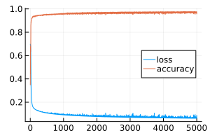
# Here is a graph that can be used to evaluate the quality of training.
gr()
plot( [ loss_history, accuracy_history], size=(300,200), label=["loss" "accuracy"], leg=:right )
Learning outcomes
We specifically saved the model's predictions before and after training:
println( "Accuracy of the forecast before training: ", 100 * mean( (probs1[1,:] .> 0.5) .== truth ), "%" )
println( "Forecast accuracy after training: ", 100 * mean( (probs2[1,:] .> 0.5) .== truth ), "%" )
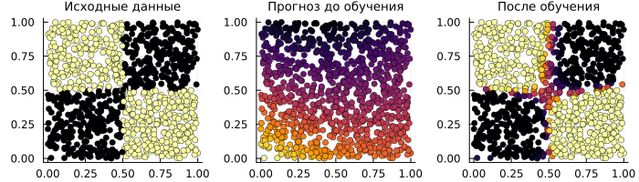
# Output a graph of the source data
p_true = scatter( inputs[1,:], inputs[2,:], zcolor=truth, title="Initial data" );
p_raw = scatter( inputs[1,:], inputs[2,:], zcolor=probs1[1,:], title="Forecast before training" );
p_done = scatter( inputs[1,:], inputs[2,:], zcolor=probs2[1,:], title="After the training" );

plot(p_true, p_raw, p_done, layout=(1,3), size=(700,200), titlefont=font(9), ms=3.5, legend=false, cbar=false )
Transferring a neural network to the Engee Function block
We will generate Julia code for this neural network by substituting symbolic variables for its input and getting a symbolic expression instead of the output.
Let's put it right inside the block Engee Function to get a block that can be copied and pasted into any other model.
# We will generate a new image to place on the front side of the block.
# (success depends on the stability of the current version of ChainPlots)

# using ChainPlots
# p = plot( model,
# titlefontsize=10, size=(300,300),
# xticks=:none, series_annotations="", markersize=8,
# markercolor="white", markerstrokewidth=4, linewidth=1 )
# savefig( p, "$(@__DIR__)/neural_net_block_mask.png");
# Creating the neural network code
using Symbolics
@variables x1 x2
s = model( [x1, x2] );
# We will load the model if it is not already open on the canvas.
if "neural_classification" ∉ getfield.(engee.get_all_models(), :name)
engee.load( "$(@__DIR__)/neural_classification.engee");
end
# The code template that we will put in the Engee Function block
code_strings = """
struct Block <: AbstractCausalComponent; end
# The neural network has two outputs: s[1] and s[2]
nn(x1, x2) = ($(s[1]), $(s[2]))
# Calculate the outputs of the neural network and return the classification result: 0 or 1
function (c::Block)(t::Real, x1, x2)
# The "probability" of each of the classes
c1, c2 = nn(x1, x2)
# Calculating the output value based on the classification results
# - if the probability of c1 is higher, the true (1) class will be selected
# - if the probability is higher than c2, then the false (2) class will be selected
return (c1 > c2) ? 1 : 0
end
"""
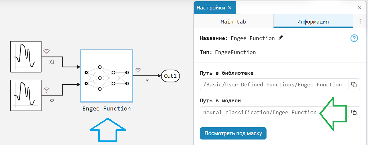
# Which block of the model should contain the neural network code?
block_address = "neural_classification/Engee Function"
engee.set_param!( block_address, "StepMethodCode" => code_strings)
# Saving the model after the change
engee.save( "neural_classification", "$(@__DIR__)/neural_classification.engee"; force = true )
The Address of the required block can be copied in the settings of this block, from the Path to Model field on the Information panel.
Let's run the model and see the result.:
model_data = engee.run( "neural_classification" );
# Prepare the output variables
model_x1 = model_data["X1"].value;
model_x2 = model_data["X2"].value;
model_y = vec( hcat( model_data["Y"].value... ));
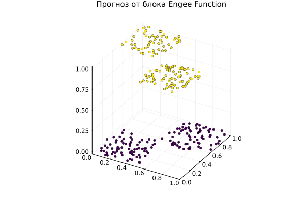
# Let's build a graph
scatter( model_x1, model_x2, model_y, ms=2.5, msw=.5, leg=false, zcolor=model_y, c=:viridis,
xlimits=(0,1), ylimits=(0,1), title="The forecast from the Engee Function block", titlefont=font(10) )
Explanation of the code
# plot( model, size=(600, 350) )
Let's look at several features of the neural network learning process for classification, namely:
- softmax function,
- one-hot encoding,
- creation of a data loader,
- loss function "cross-entropy",
- calculation of forecast accuracy.
model = Chain(
      Dense(2 => 3, tanh),
      Dense(3 => 2),
      softmax )
First, you can see that the task of our neural network is to determine which class an object should belong to.
Our neural network does not convert two input arguments into one output variable. The number of output variables is equal to the number of classes.
Please note: the last FC layer has linear activation. After it there is some "softmax layer". Softmax is an operation on numbers, which is sometimes presented as activation. But in the package Flux it is accepted otherwise. What is its essence? softmax?
Softmax translates the output values of a neural network into probabilities. These are slightly more correct inputs for the binary cross-entropy loss function (see below).
Assume that a neural network has
Nthe outputs are in the output layer, and after it is the functionsoftmax. It takes every input value.x_i, raises its exponent to a power () and for each value calculates the output . The output function divides each for the sum of all and at the output we get logits – strictly positive numbers, the sum of which is 1.
target = Flux.onehotbatch( truth, [true, false] )
Our classifier task is organized so that the network returns to us either [1, 0], or [0, 1]. Why is that?
Imagine that a neural network should return you a class number, one out of ten. If the neural network is wrong and returns 2 instead of 1, MSE returns error (2-1)=1. If the neural network is wrong and returns 10 instead of 1, MSE returns error (10-1)=9, although this error is generally not a more serious error than all the others. We need to build on something else. Coding one hot allows you to avoid comparing class numbers and compare the distribution of network "confidence" in a particular class.
But in the training sample, the values of the output variable are still scalar.: true and false. Function onehot translates them into vectors of two values: true in [1,0], and false on the vector [0,1].
data = Flux.DataLoader( (noisy, target) )
DataLoader – a slightly more elegant method of feeding data to a neural network, which does not require transposing parameter vectors before feeding them to the network. You can also pass parameters to it. shuffle = true so that the sample is mixed at each epoch of training, as well as batchsize=64 to parallelize the execution. This is what the elements that this object feeds into the neural network look like.:
data = Flux.DataLoader( (inputs, targets), batchsize=1 );
first( data )
As we have seen, the first element of the object DataLoader It consists of two parts:
- feature vector - scalar values fed to the input of the neural network,
- prediction vector - the desired class, encoded by type
one-hot.
loss(ỹ, y) = Flux.crossentropy( ỹ, y )
As mentioned above, there is a rule not to use the mean square of error (MSE) in classification tasks. Neural networks learn very slowly with it, especially if the classification is multiclass. What do we do in return?
If the classification task is organized as in our example, then cross-entropy is often used as a loss function (crossentropy), or its binary version (binarycrossentropy) if there are only two classes. Sometimes an operation is excluded from the neural network. softmax in order to speed up its operation, then you can specify that it be performed in the loss function by specifying logitcrossentropy or logitbinarycrossentropy.
accuracy(ỹ, y) = mean( Flux.onecold( ỹ ) .== Flux.onecold( y ))
We keep the accuracy of the forecast (accuracy) – the percentage of correctly guessed values. Function onecold performs the reverse operation with respect to onehot. Operation onehot-encoding finds the largest element in the vector and represents it with the number 1 in the output vector, where all other positions are 0. In turn, the operation onecold finds the largest element in the input vector and outputs a single value at the output – the class label corresponding to this element (or an ordinal number if no labels are specified).
This function can be defined much more easily, but high-level functions usually allow you to avoid a lot of errors or at least get more valuable error messages.
Not every launch leads to a good result, so at the beginning of this example, we set some specific
seed. It is useful to automatically train several models with different initialization and select the best one. Alternatively, if the training is planned to be performed very often and on a slightly different sample (as in the case of a digital twin), it is better to spend more time creating a more stable training procedure. For example, you can set up sinusoidal learning rate control or add batch normalization.
Conclusion
We trained a neural network for classification and positioned it on the canvas as another block inside the model.
The code of the training procedure is very concise, it can be reduced to 7 lines. The neural network code inside the block was generated automatically.
The code we studied for training a neural network does not have too many "hyperparameters" (parameters configurable by the designer), they can be sorted manually, and the expressive power of a multilayer neural network is very high.